Polygons Patches with Holes
Discussion: https://github.com/bokeh/bokeh/issues/2321
This document serves to specify how polygons/patches with holes could be supported in Bokeh. I'm borrowing some of the setup in the issue, but adding some extra info that helps me understand what's going on.
Right now we have Patch & Patches.
In Patch, every row is a point and the whole data source is conceptually one entity (like the state of Texas):
| x | y |
|---|---|
| 1 | 1 |
| 2 | 3 |
| 3 | 1 |
| 1 | 1 |
Show
var source = new Bokeh.ColumnDataSource({
    data: {
        x: [1, 2, 3, 1],
        y: [1, 3, 1, 1],
    }
});

var plot = Bokeh.Plotting.figure({title:'Patch', height: 300, width: 300});
var patchData = plot.patch(
    { field: "x" },
    { field: "y" },
    { source: source, fill_color: "#a6cee3" }
);
Bokeh.Plotting.show(plot, document.currentScript.parentElement);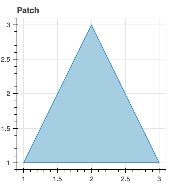
In Patches every row is a set of points and every row is its own entity (Texas, Ohio, Massachusetts...):
| xs | ys |
|---|---|
| [1, 2, 3, 1] | [1, 3, 1, 1] |
| [2, 3, 4, 2] | [2, 4, 2, 2] |
| [1, 1, 3, 3, 1] | [1, 1.5, 1.5, 1, 1] |
Show
var source = new Bokeh.ColumnDataSource({
    data: {
        xs: [[1, 2, 3, 1], [2, 3, 4, 2], [1, 1, 3, 3, 1]],
        ys: [[1, 3, 1, 1], [2, 4, 2, 2], [1, 1.5, 1.5, 1, 1]]
    }
});

var plot = Bokeh.Plotting.figure({title:'Patches', height: 300, width: 300});

var patchData = plot.patches(
    { field: "xs" },
    { field: "ys" },
    { source: source, fill_color:["limegreen", "aliceblue",  "goldenrod"]}
);
Bokeh.Plotting.show(plot, document.currentScript.parentElement);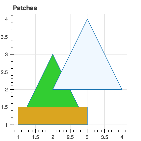
Both Patch & Patches support the idea that you can have a NaN as a data point and this will close a path and start a new one. This is useful in the case that there is an entirely separate shape that is part of another (think Michigan or Hawaii).
| x | y |
|---|---|
| 1 | 1 |
| 2 | 3 |
| 3 | 1 |
| 1 | 1 |
| Nan | NaN |
| 4 | 4 |
| 5 | 6 |
| 6 | 4 |
| 4 | 4 |
Show
var source = new Bokeh.ColumnDataSource({
    data: {
        xs: [1, 2, 3, 1, NaN, 4, 5, 6, 4],
        ys: [1, 3, 1, 1, NaN, 4, 6, 4, 4],
    }
});

var plot = Bokeh.Plotting.figure({title:'MultiPatch (NaN separated)', height: 300, width: 300});
var patchData = plot.patch(
    { field: "xs" },
    { field: "ys" },
    { source: source, fill_color: "#a6cee3" }
);
Bokeh.Plotting.show(plot,document.currentScript.parentElement);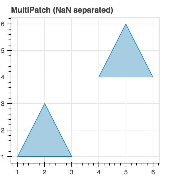
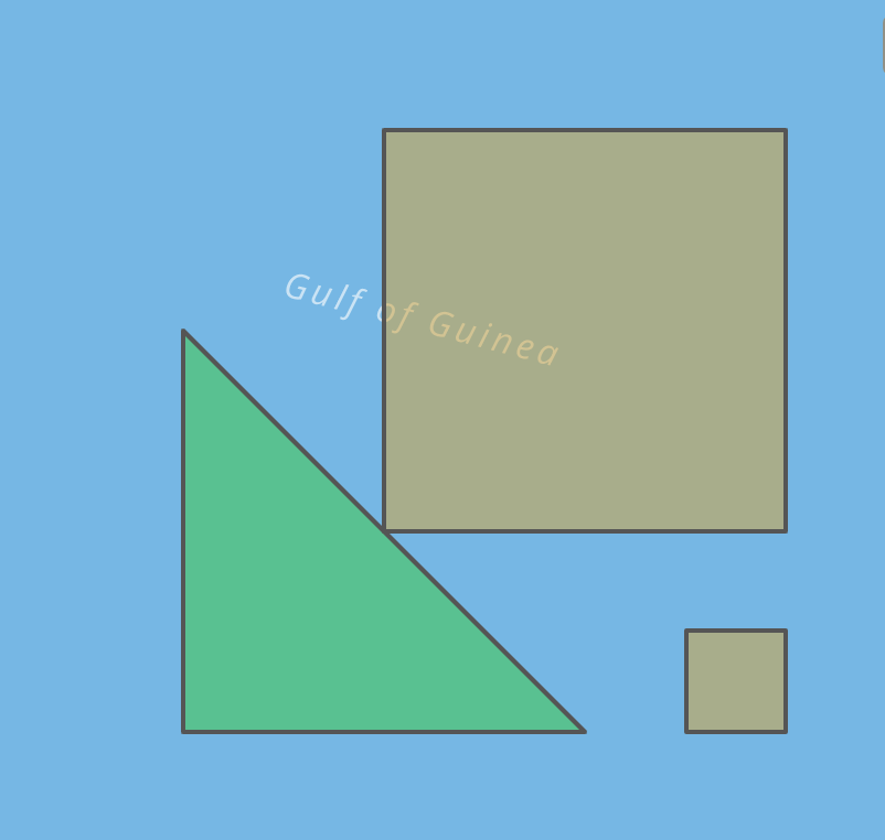
| xs | ys | color |
|---|---|---|
| [1, 1, 3] | [1, 3, 1] | 'limegreen' |
| [2, 2, 4, 4, NaN, 3.5, 3.5, 4, 4] | [2, 4, 4, 2, NaN, 1, 1.5, 1.5, 1] | 'goldenrod' |
Show
var source = new Bokeh.ColumnDataSource({
    data: {
        xs: [[1, 1, 3], [2, 2, 4, 4, NaN, 3.5, 3.5, 4, 4]],
        ys: [[1, 3, 1], [2, 4, 4, 2, NaN, 1, 1.5, 1.5, 1]],
    }
});

var plot = Bokeh.Plotting.figure({title:'MultiPatches (NaN separated)', height: 300, width: 300});
var patchData = plot.patches(
    { field: "xs" },
    { field: "ys" },
    { source: source, fill_color:['limegreen', 'goldenrod']}
);
Bokeh.Plotting.show(plot,document.currentScript.parentElement);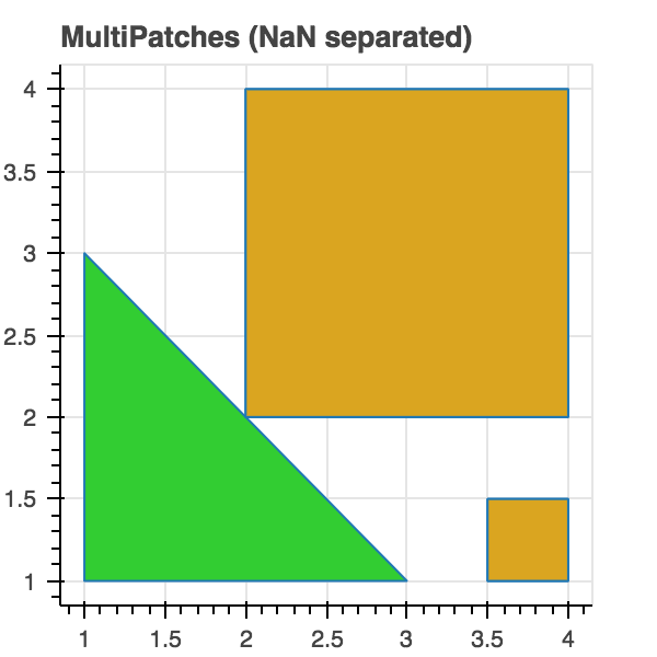
GeoJSON takes a more nested approach.
http://geojson.org/geojson-spec.html#id4
Coordinates of a Polygon are an array of LinearRing coordinate arrays. The first element in the array represents the exterior ring. Any subsequent elements represent interior rings (or holes).
No holes:

{ "type": "Polygon",
    "coordinates": [
      [ [100.0, 0.0], [101.0, 0.0], [101.0, 1.0], [100.0, 1.0], [100.0, 0.0] ]
      ]
   }

With holes:

{ "type": "Polygon",
    "coordinates": [
      [ [100.0, 0.0], [101.0, 0.0], [101.0, 1.0], [100.0, 1.0], [100.0, 0.0] ],
      [ [100.2, 0.2], [100.8, 0.2], [100.8, 0.8], [100.2, 0.8], [100.2, 0.2] ]
      ]
}http://geojson.org/geojson-spec.html#id7
Coordinates of a MultiPolygon are an array of Polygon coordinate arrays:
{ "type": "MultiPolygon",
    "coordinates": [
      [[[102.0, 2.0], [103.0, 2.0], [103.0, 3.0], [102.0, 3.0], [102.0, 2.0]]],
      [[[100.0, 0.0], [101.0, 0.0], [101.0, 1.0], [100.0, 1.0], [100.0, 0.0]],
       [[100.2, 0.2], [100.8, 0.2], [100.8, 0.8], [100.2, 0.8], [100.2, 0.2]]]
   ]
}Each bokeh Patch corresponds to a MultiPolygon in geoJSON and Patches corresponds to a FeatureCollection of MultiPolygons. In practice it is generally fine to lump together the functionality on MultiPolygons and Polygons, but if we want to preserve all the information conveyed by
| xs | ys | color |
|---|---|---|
| [1, 1, 3, 3] | [1, 3, 1, 1] | 'limegreen' |
| [2, 2, 4, 4, NaN, 3.5, 3.5, 4, 4] | [2, 4, 4, 2, NaN, 1, 1.5, 1.5, 1] | 'goldenrod' |
is equivalent to
{
  "type": "FeatureCollection",
  "features": [{
    "type": "Feature",
    "properties": {
      "fill": "limegreen"
    },
    "geometry": {
      "type": "Polygon",
      "coordinates": [
        [[1, 1], [1, 3], [3,1], [1, 1]]
      ]
    }
  },
  {
    "type": "Feature",
    "properties": {
      "fill": "goldenrod"
    },
    "geometry": {
      "type": "MultiPolygon",
      "coordinates": [
        [[[2, 2], [2, 4], [4, 4], [4, 2], [2, 2]]],
        [[[3.5, 1], [3.5, 1.5], [4, 1.5], [4, 1], [3.5, 1]]]
     ]
    }
  }]
}
Try it out at http://geojson.io/#map=7/2.5/2.5
In geoJSON each array of holes is relative to a Polygon not a MultiPolygon. So, in bokeh, in order to not lose information we'd need to have a list of holes for each NaN separated array in a Patch. So we will have some information loss if we keep using NaN separation, but that might be ok as long as we can still draw the shape properly.
{
  "type": "FeatureCollection",
  "features": [{
    "type": "Feature",
    "properties": {
      "fill": "red"
    },
    "geometry": {
      "type": "Polygon",
      "coordinates": [
        [[1, 4], [1, 3], [2,3], [2,4], [1, 4]]
      ]
    }
  },
  {
    "type": "Feature",
    "properties": {
      "fill": "limegreen"
    },
    "geometry": {
      "type": "Polygon",
      "coordinates": [
        [[1, 1], [3, 1], [1, 3], [1, 1]],
        [[1.5, 1.5], [1.5, 2], [2, 1.5], [1.5,1.5]]
      ]
    }
  },
  {
    "type": "Feature",
    "properties": {
      "fill": "goldenrod"
    },
    "geometry": {
      "type": "MultiPolygon",
      "coordinates": [
        [
          [[2, 2], [4, 2], [4, 4], [2, 4], [2, 2]],
          [[2.5, 3], [2.5, 3.5], [3, 3.5], [2.5, 3]],
          [[3.5, 2.5], [3, 2.5], [3, 3], [3.5, 3], [3.5, 2.5]]
        ],
        [
          [[3.5, 1], [4, 1], [4, 1.5], [3.5, 1.5], [3.5, 1]]
        ]
     ]
    }
  }]
}
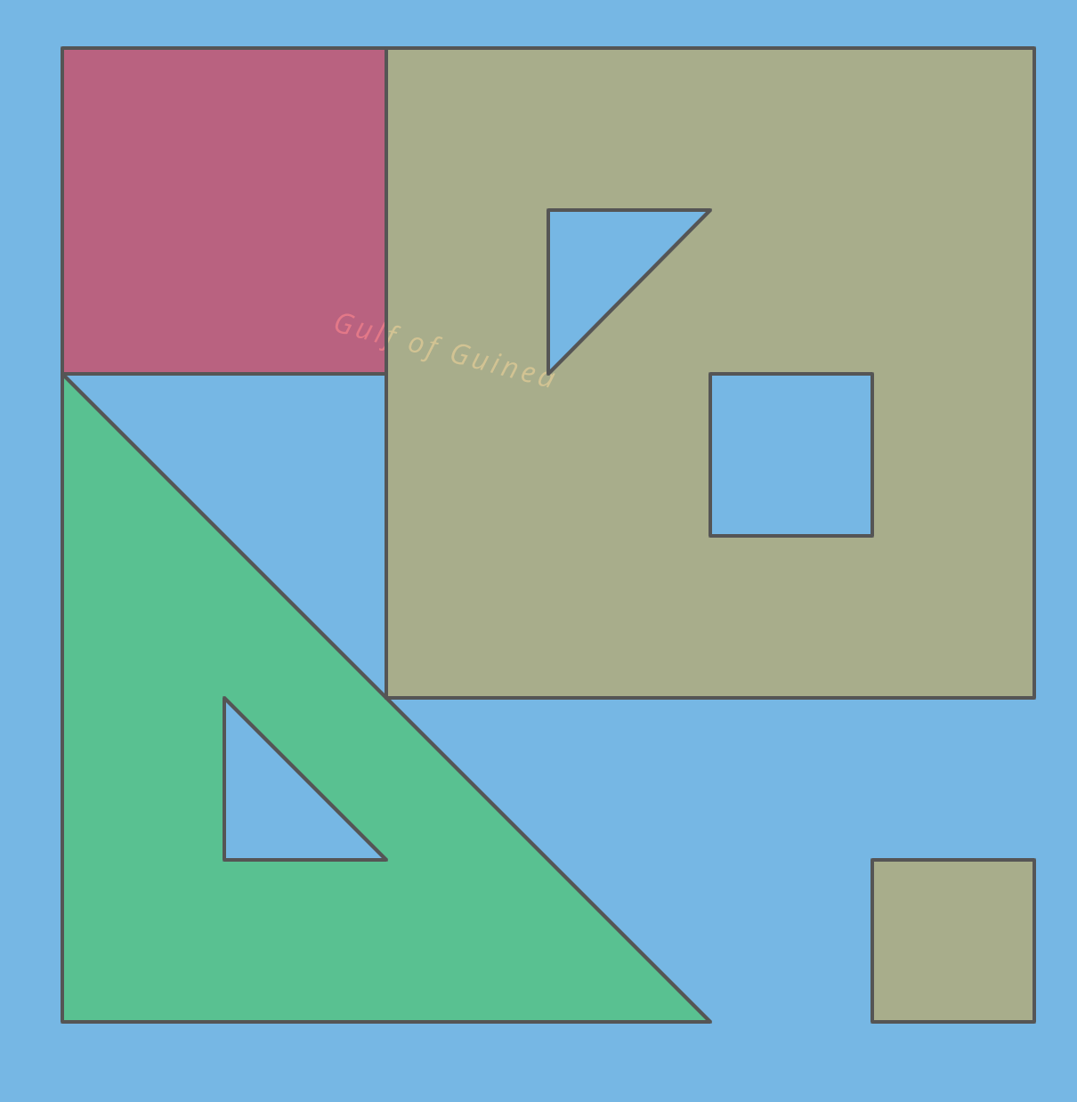
So the first thought is that we could allow the passing a list of holes for each row:
| xs | ys | hole_x | hole_y | color |
|---|---|---|---|---|
| [1, 1, 2, 2] | [4, 3, 3, 4] | 'red | ||
| [1, 1, 3] | [1, 3, 1] | [1.5, 1.5, 2] | [1.5, 2, 1.5] | 'limegreen' |
| [2, 2, 4, 4, NaN, 3.5, 3.5, 4, 4] | [2, 4, 4, 2, NaN, 1, 1.5, 1.5, 1] | [2.5, 2.5, 3], [3.5, 3, 3, 3.5] | [3, 3.5, 3.5], [2.5, 2.5, 3, 3] | 'goldenrod' |
var source = new Bokeh.ColumnDataSource({
    data: {
        xs: [[1, 1, 2, 2], [1, 1, 3], [2, 2, 4, 4, NaN, 3.5, 3.5, 4, 4]],
        ys: [[4, 3, 3, 4], [1, 3, 1], [2, 4, 4, 2, NaN, 1, 1.5, 1.5, 1]],
        hole_xs: [[[]], [[1.5, 1.5, 2]], [[2.5, 2.5, 3], [3.5, 3, 3, 3.5]]],
        hole_ys: [[[]], [[1.5, 2, 1.5]], [[3, 3.5, 3.5], [2.5, 2.5, 3, 3]]]
    }
});

var plot = Bokeh.Plotting.figure({title:'MultiPatches with Holes using Column', height: 300, width: 300});
var patchData = plot.patches(
    { field: "xs" },
    { field: "ys" },
    { field: "hole_xs" },
    { field: "hole_ys" },
    { source: source, fill_color:['red', 'limegreen', 'goldenrod']}
);
Bokeh.Plotting.show(plot,document.currentScript.parentElement);Another option would be to have a ColumnData for hole_xs, and hole_ys indexed by the row of Patches. This has the benefit of being less sparse, but the downside of being less tightly tied to the data, so that if the Patches get sorted or filtered, the hole_xs and hole_ys may no longer align.
| xs | ys | color |
|---|---|---|
| [1, 1, 2, 2] | [4, 3, 3, 4] | 'red |
| [1, 1, 3] | [1, 3, 1] | 'limegreen' |
| [2, 2, 4, 4, NaN, 3.5, 3.5, 4, 4] | [2, 4, 4, 2, NaN, 1, 1.5, 1.5, 1] | 'goldenrod' |
hole_xs = {1: [[1.5, 1.5, 2]], 2: [[2.5, 2.5, 3], [3.5, 3, 3, 3.5]]}
hole_ys = {1: [[1.5, 2, 1.5]], 2: [[3, 3.5, 3.5], [2.5, 2.5, 3, 3]]}
var source = new Bokeh.ColumnDataSource({
data: {
xs: [[1, 1, 2, 2], [1, 1, 3], [2, 2, 4, 4, NaN, 3.5, 3.5, 4, 4]],
ys: [[4, 3, 3, 4], [1, 3, 1], [2, 4, 4, 2, NaN, 1, 1.5, 1.5, 1]],
}
});
var hole_xs = {1: [[1.5, 1.5, 2]], 2: [[2.5, 2.5, 3], [3.5, 3, 3, 3.5]]};
var hole_ys = {1: [[1.5, 2, 1.5]], 2: [[3, 3.5, 3.5], [2.5, 2.5, 3, 3]]};
var plot = Bokeh.Plotting.figure({title:'MultiPatches with Holes using Dict', height: 300, width: 300});
var patchData = plot.patches(
{ field: "xs" },
{ field: "ys" },
{ source: source, fill_color:['red', 'limegreen', 'goldenrod'], hole_xs: hole_xs, hole_ys: hole_ys}
);
Bokeh.Plotting.show(plot,document.currentScript.parentElement);For Patch this would look like:
| x | y |
|---|---|
| 1 | 1 |
| 2 | 3 |
| 3 | 1 |
| 1 | 1 |
hole_xs = [[1.5, 1.5, 2]]
hole_ys = [[1.5, 2, 1.5]]The new glyph would implement nesting in the same manner as geoJSON does, with the holes on each polygon part. Notice that this is more annoying the write the data sources like this, but the user interface is cleaner. So this mechanism expects users to be loading data rather than writing their own.
var source = new Bokeh.ColumnDataSource({
    data: {
        xs: [
            [
                [[1, 1, 2, 2]],
            ],
            [
                [[1, 1, 3], [1.5, 1.5, 2]]
            ],
            [
                [[2, 2, 4, 4], [2.5, 2.5, 3], [3.5, 3, 3, 3.5]],
                [[3.5, 3.5, 4, 4]]
            ]
        ],
        ys: [
            [
                [[4, 3, 3, 4]],
            ],
            [
                [[1, 3, 1], [1.5, 2, 1.5]],
            ],
            [
                [[2, 4, 4, 2], [3, 3.5, 3.5], [2.5, 2.5, 3, 3]],
                [[1, 1.5, 1.5, 1]]
            ]
        ]
    }
});

var plot = Bokeh.Plotting.figure({title:'New Glyph - Polygons with Holes', height: 300, width: 300});
var patchData = plot.polygons(
    { field: "xs" },
    { field: "ys" },
    { source: source, fill_color:['red', 'limegreen', 'goldenrod']}
);

Bokeh.Plotting.show(plot,document.currentScript.parentElement);There are basically two options for this - we can use winding and the right hand rule to draw counterclockwise for Patches and clockwise for holes. This approach has the benefit of being explicit and the geoJSON spec does specify that values should be saved in this order (https://tools.ietf.org/html/rfc7946#section-3.1.6). However direction of storage isn't enforced, since the former geoJSON spec didn't enforce (or mention) winding. So geoJSON can be valid and have the wrong winding direction for holes we can mimic geopandas/matplotlib and not draw the holes in these cases, or we can reverse the direction.
Another option would be to use the "evenodd" fillRule. The down-side of this is that we would need to check that holes are contained in the polygons so that the fill does not get inverted. Similar worries crop up when wholes overlap creating a odd number of layers (shapely throws errors for those kinds of situations). I'd also be worried about browser compatibility for using the fillRule.
Another thing to keep in mind is that all drawing for a particular polygon has to be done before the fill occurs. This means that we will need to do something slightly different when we split on nans. Instead of filling each nan separated part of the patch as we go, we will need to just close the path and fill them whole patch at the end.