DiscoPlot

DiscoPlot allows the user to quickly identify genomic rearrangements, misassemblies and sequencing artefacts by providing a scalable method for visualising large sections of the genome. It reads single-end or paired read alignments in SAM, BAM or standard BLAST tab format and creates a scatter plot of opaque crosses representing the alignments to a reference. DiscoPlot is freely available (under a GPL license) for download (Mac OS X, Unix and Windows) at: https://github.com/BeatsonLab-MicrobialGenomics/DiscoPlot/releases.

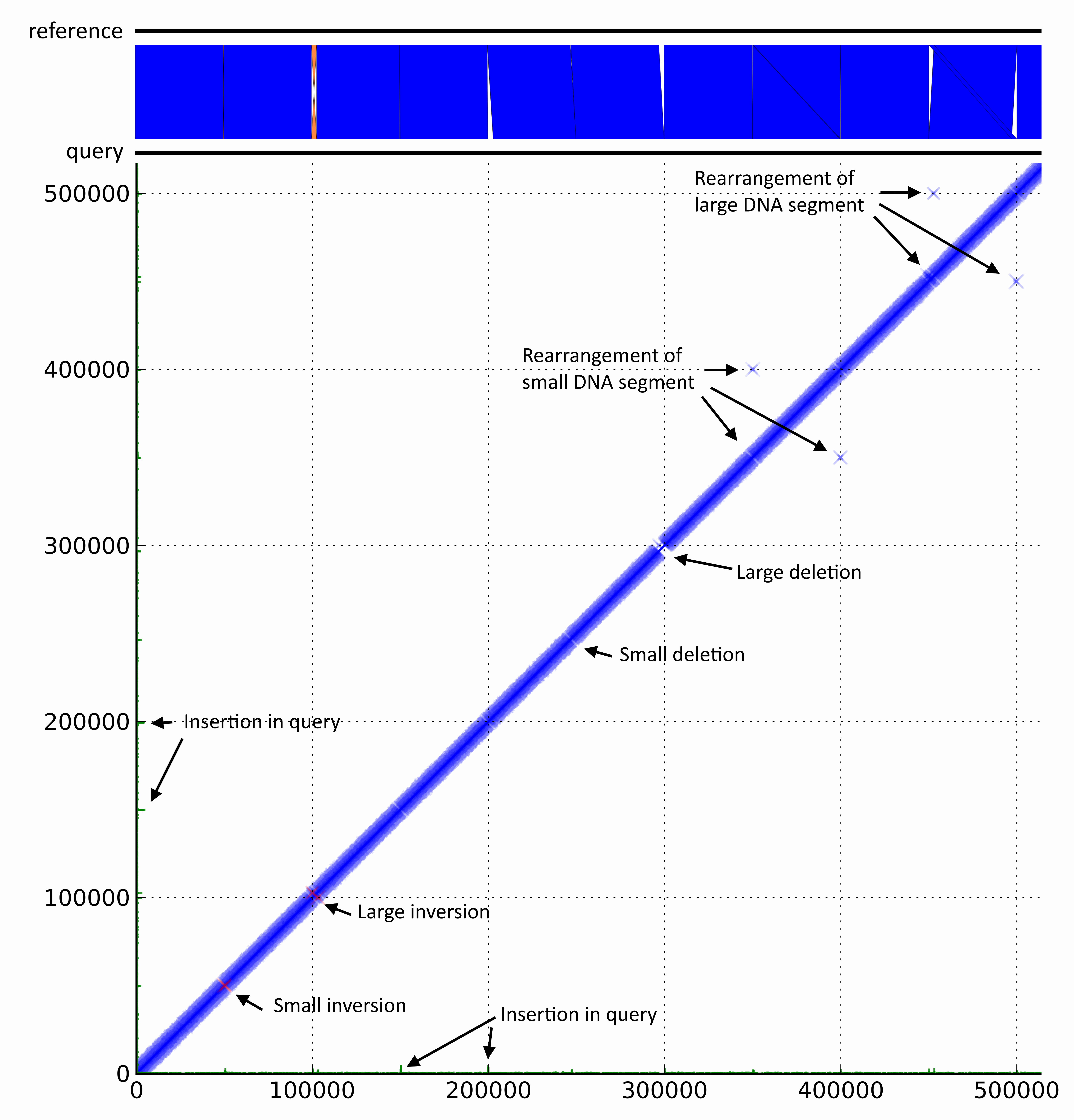
DiscoPlot of a mock genome. A mock genome was created by adding genomic rearrangements to the chromosome of E. coli str. UTI89. Paired-end reads generated from the mock genome (query) with GemSim and mapped back to UTI89 (reference). The first ~500 Kbp were then visualised using DiscoPlot.

Table of Contents

Documentation

Please use this README.rst as the core DiscoPlot user documentation.

Citation

Cite this Github repository if you use DiscoPlot to generate figures for publications:

SULLIVAN MJ & BEATSON SA^. 
DiscoPlot - Visualising discordant reads.
https://github.com/BeatsonLab-MicrobialGenomics/DiscoPlot.

TODO

On the roadmap:

• Print selected read names, alignments or sequences

Installation

DiscoPlot is a commandline application. If you're not familiar with the commandline we recommend you ask local IT support to help you install it.

You will need to install/have installed:

• python >= 2.7 (Python 3 is not supported)

To automatically generate BLAST aligments (For long read DiscoPlots) using DiscoPlot you will need to install/have installed:

• ncbiblast+ >= 2.2.27

You can check these are installed by:

$ python --version
$ blastn -version

Installation of python or blastn (without a package manager) is beyond the scope of this document.

If you have both python and blastn you need to (if not already present) install pip.

You can check if pip exists with:

$ which pip

If you get a "not found", please read the pip installation instructions.

If you already have pip we do suggest you upgrade it. We are using version 1.5.6 at the time of writing this document.

You can upgrade pip like this:

$ pip install --upgrade pip

The following python libraries should be installed (automatically) if you follow the installation instructions detailed below.

We use the following python libraries:

• numpy >= 1.8.1
• matplotlib >= 1.3.1
• pysam >= 0.8.1

Pysam is only required for generating DiscoPlots with BAM files. SAM compatability has been included to allow windows users to generate DiscoPlots. PySam will not install on Windows, don't bother trying (or if you've succeeded please let me know how).

Linux (Ubuntu)

Discoplot uses 3rd party packages that are extremely important for scientific computing but may be difficult to install. While pip install --user DiscoPlot may work we recommend you install these 3rd party packages using apt-get.

Run:

$ sudo apt-get install python-numpy python-matplotlib 

Now pip install DiscoPlot:

$ pip install --user DiscoPlot

We use the --user option of pip to put DiscoPlot in: /home/$USER/.local/bin/ You need to add this location to you ~/.bash_profile.

Add DiscoPlot to your path:

$ echo 'export PATH=$PATH:/home/$USER/.local/bin/' >> ~/.bash_profile

Finally install BLAST+:

$ sudo apt-get install ncbi-blast+ 

MacOSX (Mavericks)

You'll need to have the equivalents of python-dev libatlas-dev liblapack-dev gfortran libfreetype6-dev libfreetype6 & libpng-dev installed. We had no problems installing DiscoPlot on a recently acquired OSX Mavericks machine using the homebrew package manager.

The installed packages on this machine via:

$ brew list 

Are available at this gist.

pip install DiscoPlot:

$ pip install --user DiscoPlot

We use the --user option of pip to put DiscoPlot in: /Users/$HOME/Library/Python/2.7/bin You need to add this location to you ~/.bash_profile.

Add DiscoPlot to your path:

$ echo 'export PATH=$PATH:/Users/$HOME/Library/Python/2.7/bin/ >> ~/.bash_profile'

Finally install BLAST+:

$ sudo brew install blast 

Windows

Download and install numpy and matplotlib. To make this process easier you can download a distribution of python with matplotlib and numpy already installed such as anaconda.

pip install DiscoPlot:

$ pip install DiscoPlot

Finally download and install BLAST.

Testing DiscoPlot Installation

Run:

$ DiscoPlot -h 
$ python -c 'import DiscoPlot; print DiscoPlot'

Upgrading DiscoPlot

You can upgrade like this:

pip install --upgrade DiscoPlot

Please regularly check back to make sure you're running the most recent DiscoPlot version.

Examples

DiscoPlot of a mock genome. A mock genome was created by adding genomic rearrangements to the chromosome of E. coli str. UTI89. Paired-end reads generated from the mock genome (query) with GemSim (ref) and mapped back to UTI89 (reference). The first ~500 Kbp were then visualised using DiscoPlot.

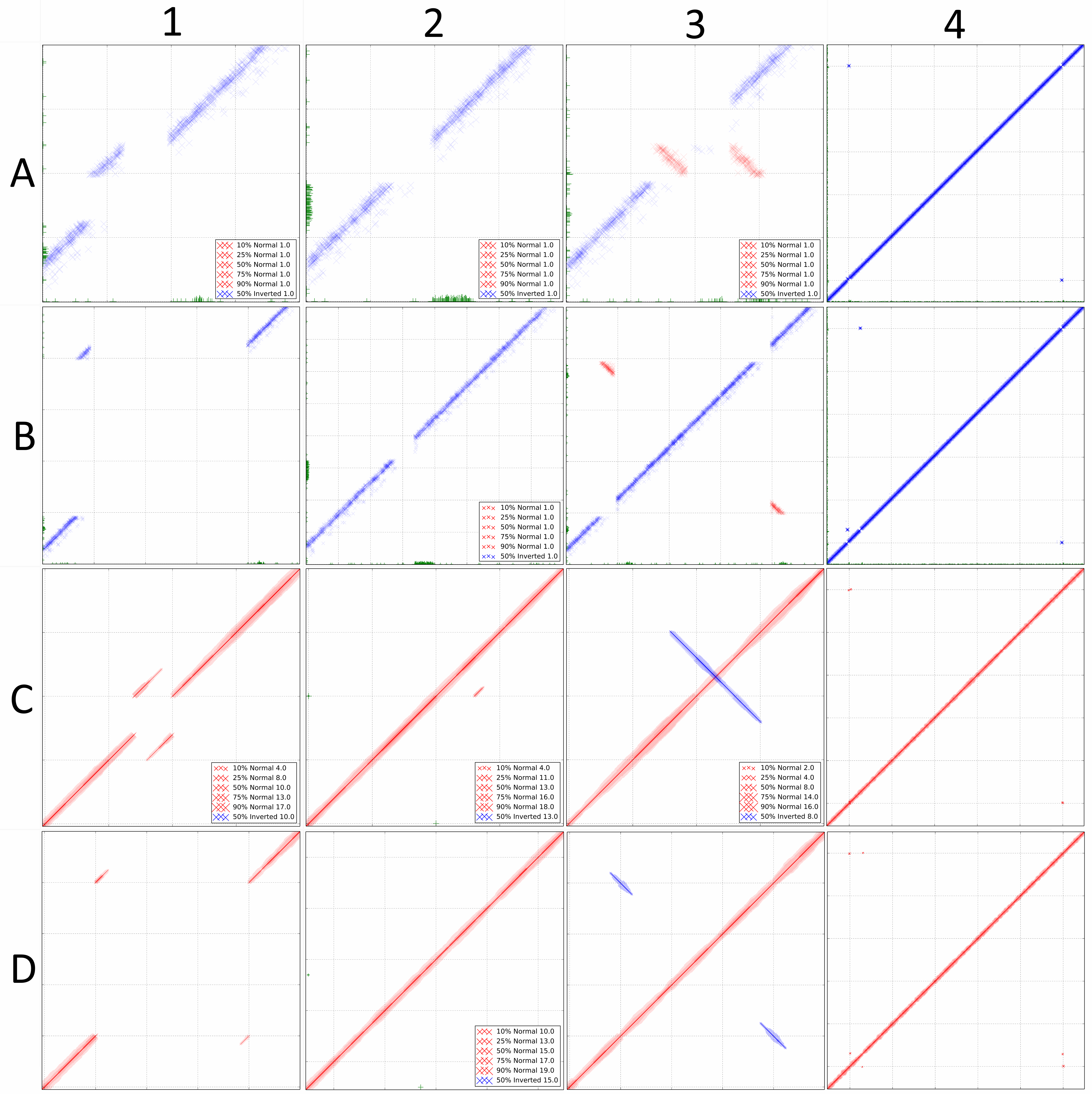
DiscoPlots of common structural variants. Each box shows a common genomic rearrangement represented by a DiscoPlot. Rows A and B were created using 100 bp long paired-end reads with an insert size of 300bp. Rows C and D were created using single-end reads with an average length of 1000bp. For each box the rearrangement in the sequenced genome is listed, followed by the scale of the gridlines in brackets. A1, C1: 300 bp deletion (400 bp). A2, C2: 300 bp insertion (400 bp). A3, C3: 300 bp inversion (400 bp). A4, C4: 300 bp sequence translocated 50 Kbp upstream (10 Kbp). B1, D1: 3000 bp deletion (1000 bp). B2, D2: 3000 bp insertion (500 bp). B3, D3: 3000 bp inversion (1000 bp). B4, D4: 3000 bp sequence translocated 50 Kbp upstream (10 Kbp).

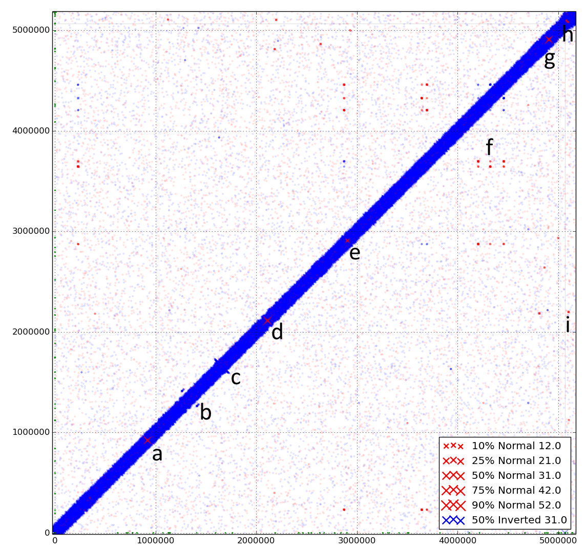
The dynamic nature of the genome of Escherichia coli str. UTI89. Discoplot of paired-end reads from a clonal culture of UTI89 mapped back to the published reference chromosome and plasmid. Coordinates from 0 to 5,065,741 represent the chromosome of E. coli UTI89, coordinates ≥ 5,066,000 represent the plasmid of E. coli UTI89

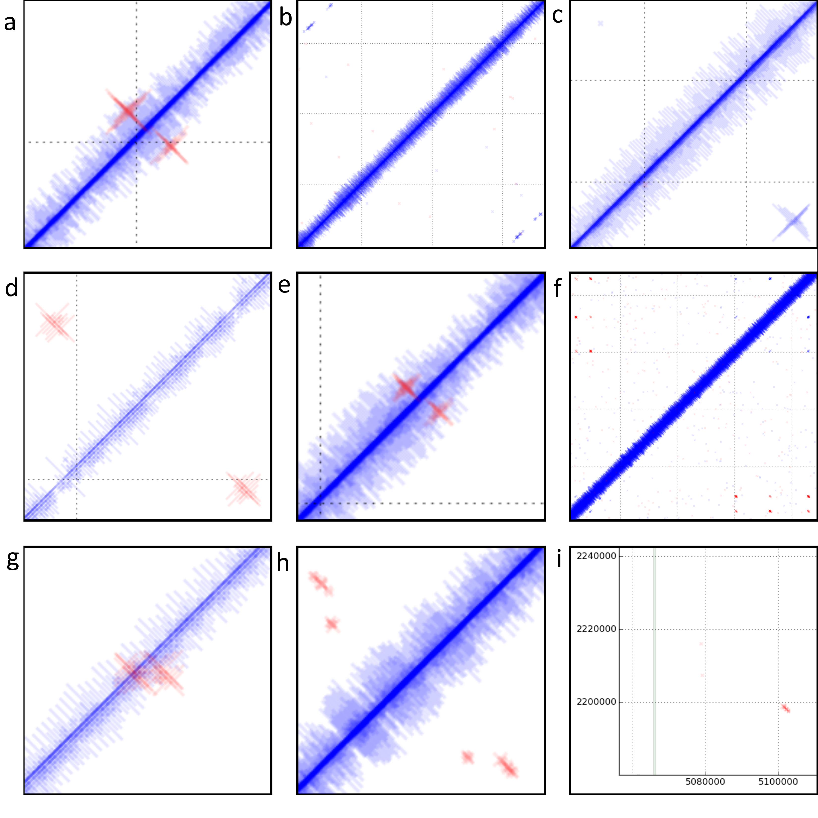
Discordant reads in E. coli str. UTI89. a) Read alignment indicates inversion of bases 919,638..922,323. 12bp inverted repeat present at terminals of region. Start and stop of inverted region occurs in two probable tail fibre proteins. Two additional tail fibre assembly proteins are encoded within the boundaries of this region. Region is immediately downstream of a putative DNA invertase gene. b, f, h, i) Reads are misaligned as they map equally well in a concordant position. c) Read alignment indicates circularisation of bases 1,653,000..1,662,603. 17bp direct repeats present at terminals of this region. Region also encodes five putative phage-related membrane proteins, two putative phage proteins, three phage hypothetical proteins, four hypothetical proteins and a single putative phage related secreted protein. Size of crosses indicates coverage of this region is higher than average. Only a single read (indicated by the cross, top left) indicates potential excision of this region. d) Read alignments indicate inversion of bases 2,109,690..2,114,003. Region contains ~100bp inverted repeat at terminals which encodes a tRNA. Region contains 3 hypothetical proteins and an additional tRNA identical to the repeats. A P4-phage integrase is present immediately downstream of the inversion. The lack of concordantly mapping reads at prophage boundary indicates that the inverted phage has reached fixation in the population. e) Reads indicate inversion of bases 2,906,008..2,906,936. 15bp inverted repeats present at terminals of this region. The 3’ end of a putative tail fibre assembly gene is encoded by this region. g) Read alignments indicate inversion of bases 4,907,424..4,907,737. Regions has 9bp inverted repeat at terminals. It is located in a non-coding region between fimA and fimE which encode the type I fimbriae.

Tutorials

Quick Start - paired-end/mate-pair short reads.

Align reads with your favourite short read aligner (e.g. BWA, Bowtie2)

Create DiscoPlot from sam file with 5000 bins - open in a matplotlib window:

DiscoPlot.py -sam sam_file.sam -s 5000 

Create a DiscoPlot from a bam file using a bin size of 10,000bp - save as .png file:

DisocPlot.py -bam bam_file.bam -bin 10000 -o discoplot.png

Quick Start - long reads

To automatically generate a BLAST alignment using BLAST+ run:

DiscoPlot.py -r reads.fa -ref reference.fasta -B -s 5000 

To provide DiscoPlot with an alignment file (BLAST tab delimited format):

DiscoPlot -ref reference.fasta -b alignment.out -s 5000 

More Coming Soon

Using DiscoPlot

DiscoPlot.py - Visualising discordant reads.

In paired read mode DiscoPlot must be provided with a BAM or SAM file. In Single read mode DiscoPlit must be provided with a alignment file (BLAST tab delimited format) or reads and a reference (in FASTA format).

-bin (size of bins in bp) or -s (size of bins) must be specified.

additional arguments:

-h, --help            show this help message and exit
-r READ_FILE, --read_file READ_FILE
                      read file - provide DiscoPlot with a read file to
                      BLAST (long read mode).
-ref REFERENCE_FILE, --reference_file REFERENCE_FILE
                      Reference file - Reference for generating long reads
                      alignments.
-bam BAM_FILE, --bam_file BAM_FILE
                      bam file - paired read mode. (Requires pysam).
-sam SAM_FILE, --sam_file SAM_FILE
                      sam file - paired read mode. (pysam not required)
-hm HEATMAP, --heatmap HEATMAP
                      Heatmap file - provide DiscoPlot with custom generated
                      heatmap.
-B GEN_BLAST, --gen_blast GEN_BLAST
                      Generate blast files, use argument as prefix for
                      output.
-b BLAST_FILE, --blast_file BLAST_FILE
                      Provide DiscoPlot with alignment file (long read mode)
                      (BLAST tab delimited file - output format 6)
-o OUTPUT_FILE, --output_file OUTPUT_FILE
                      output file [gif/bmp/png]
-s SIZE, --size SIZE  Number of bins.
-bin BIN_SIZE, --bin_size BIN_SIZE
                      Bin size (in bp)
-g GAP, --gap GAP     Gap size - gap size between entries in reference.
-sub SUBSECTION [SUBSECTION ...], --subsection SUBSECTION [SUBSECTION ...]
                      Only display subection of genome [ref]/[min_cutoff
                      max_cutoff]/[ref min_cutoff max_cutoff]
-wb WRITE_READS [WRITE_READS ...], --write_reads WRITE_READS [WRITE_READS ...]
                      Write reads in rectangle to bam/sam [x1 y1 x2 y2
                      out.bam]
-c MIN_HITS, --min_hits MIN_HITS
                      Only show bins with more than this number of hits.
-m MAX_HITS, --max_hits MAX_HITS
                      Only show bins with less hits than this.
-dpi IMAGE_QUALITY, --image_quality IMAGE_QUALITY
                      Image quality (in DPI)
-i MIN_IDENT, --min_ident MIN_IDENT
                      Min. idenity of hits to draw (long read mode).
-l MIN_LENGTH, --min_length MIN_LENGTH
                      Min. length of hits to draw (long read mode).
-d UNMAPPED, --unmapped UNMAPPED
                      Unmapped bases on edge for RMaD to consider read
                      partially unmapped.
-a ALPHA, --alpha ALPHA
                      Transparency of mapped read markers
-a2 ALPHA2, --alpha2 ALPHA2
                      Transparency of unmapped read markers
-mc M_COUNT, --m_count M_COUNT
                      The count of a bin to be used as the median value for
                      calculating the size of the dot [auto]
-ms M_SIZE, --m_size M_SIZE
                      Set the width (in bins) of a marker with a median
                      count.
-log, --log           Log10 bin counts. (For data with highly variable
                      coverage).
-sw, --switch         Draw most common (inverted/direct) hits first.
-nl, --no_legend      Don't create legend.
-ng, --no_gridlines   Don't draw gridlines.
-na, --no_label       No axis labels.
-split SPLIT_GRAPH [SPLIT_GRAPH ...], --split_graph SPLIT_GRAPH [SPLIT_GRAPH ...]
                      Show multiple subsections of graph [start1 stop1
                      start2 stop2 etc.] or [ref1 start1 stop1 ref2 start2
                      stop2 etc.]
-hl HIGHLIGHT [HIGHLIGHT ...], --highlight HIGHLIGHT [HIGHLIGHT ...]
                      Highlight subsections of graph [alpha start1 stop1
                      start2 stop2 etc.] or [alpha ref1 start1 stop1 ref2
                      start2 stop2 etc.]
-mw MARKER_EDGE_WIDTH, --marker_edge_width MARKER_EDGE_WIDTH
                      Marker width (default is roughly 20x bin size)

Thanks for using DiscoPlot.py