![]()
Epilogos is an approach for analyzing, visualizing, and navigating multi-biosample functional genomic annotations, with an emphasis on chromatin state maps generated with e.g. ChromHMM or Segway.
The software provided in this repository implements the methods underlying Epilogos using Python 3.9. We provide a proof-of-principle dataset based on chromatin state calls from the EpiMap dataset (Boix et al., Nature 2021).
Created by: Wouter Meuleman, Jacob Quon, Alex Reynolds, and Eric Rynes
Although not required, it is good practice to create a virtual environment in which
specific versions of Python and its libraries are installed.
This can be done using conda, for instance as such:
$ conda init bash  ## only needed upon first use of conda. Restart shell after this.
$ conda create -n epilogos python=3.9
$ conda activate epilogos
To install Epilogos simply run the following two commands
$ pip install epilogosAlternatively, install Epilogos directly from this Git repository using
$ pip install git+https://github.com/meuleman/epilogosTo compute epilogos, you will need to have the following python libraries installed: statsmodels, click, numpy, scipy, matplotlib, pandas, pysam, scikit-learn, natsort, pyranges, and rich. In case the abovementioned commands not automatically and correctly take care of this, the libraries can be installed with one of the following commands.
$ pip install 'click==8.1.3' 'numpy==1.23.4' 'pandas==1.5.1' 'scipy==1.9.3' 'matplotlib==3.6.1' 'statsmodels==0.13.2' 'scikit-learn==1.1.3' 'pysam==0.19.1' 'natsort==8.2.0' 'pyranges==0.0.117' 'rich==12.6.0'or while in the epilogos directory
$ pip install -r requirements.txtAdditionally, it is recommended that python is updated to version 3.9 or later. We cannot guarantee the validity of results generated by earlier verions of python.
To be presented with basic documentation of arguments needed to run epilogos, simply run the command epilogos --help or python -m epilogos --help (More in-depth explanation is given below).
By default, Epilogos assumes access to a computational cluster managed by SLURM.
A version of epilogos has been created for those without access to a SLURM cluster and can be run by using the -l flag to your command (e.g. epilogos -l).
Minimal example on provided example data
If you cloned this git repository, example data has been provided under data/pyData/male/. Otherwise it is available for download using the script in bin/download_example_data.sh. The script uses cURL to download neccessary files and places them in a file hierarchy generated within the current directory.
The file, epilogos_matrix_chr1.txt.gz, contains chromatin state calls for a 18-state chromatin model, across 200bp genomic bins spanning human chromosome 1.
The data was pulled from the EpiMap dataset and contains only those epigenomes which are tagged Male under the Sex column.
To compute epilogos (using the S1 saliency metric) for this sample data run following command within the epilogos/ directory (replacing OUTPUTDIR with the output directory of your choice).
$ epilogos -i data/pyData/male/ -j data/state_metadata/human/Boix_et_al_833_sample/hg19/18/metadata.tsv -o OUTPUTDIRUpon completion of the run, you should see the files scores_male_s1_epilogos_matrix_chr1.txt.gz and regionsOfInterest_male_s1.txt in OUTPUTDIR
To customize your run of epilogos see the Command Line Options of the README
Running Epilogos with your own data
Before you can run Epilogos on your own data, you will need to complete two steps.
First, you will need to format your data such that Epilogos can parse it.
To assist with this, we have provided a bash script which takes ChromHMM files and generates Epilogos input files.
This can be found at scripts/preprocess_data_ChromHMM.sh (to get usage information, run without arguments).
If you would prefer not to use the script, data is to be formatted as follows:
Column 1: Chromosome name
Column 2: Start coordinate
Column 3: End coordinate
Column 4: State data for epigenome 1
...
Column n: State data for epigenome n-3
Second, you will need to create a state info file.
This is a tab separated file containing various information about each of the states in the chromatin state model.
We have provided some files already for common models in the data/state_metadata/ directory.
For more information on the structure of these files see data/state_metadata/README.txt or State Info [-j, --state-info]
Once you have completed these two steps, you can run epilogos with the following command:
$ epilogos -i PATH/TO/INPUT_DIR -j PATH/TO/STATE_INFO_TSV -o PATH/TO/OUTPUT_DIRUpon completion of the run, you should see the same number of scores files as in your input directory in OUTPUTDIR.
Each of these files will be named scores_*.txt.gz, where 'scores_' is followed by the input directory name, the saliency metric, and the corresponding input file name (extensions removed).
Additionally, you will find a regionsOfInterest_*.txt file which follows the same naming convention minus the input file name.
If you would like to visualize these results as seen on epilogos.altius.org, we recommend using higlass.
To further customize your run of epilogos see the Command Line Options of the README
Minimal example on provided example data
If you cloned this git repository, example data has been provided under data/pyData/male/. Otherwise it is available for download using the script in bin/download_example_data.sh. The script uses cURL to download neccessary files and places them in a file hierarchy generated within the current directory.
The file, epilogos_matrix_chr1.txt.gz, contains chromatin state calls for a 18-state chromatin model, across 200bp genomic bins spanning human chromosome 1.
The data was pulled from the EpiMap dataset and contains only those epigenomes which are tagged Male under the Sex column.
To compute epilogos (using the S1 saliency metric) for this sample data run following command within the epilogos/ directory (replacing OUTPUTDIR with the output directory of your choice).
$ epilogos -l -i data/pyData/male/ -j data/state_metadata/human/Boix_et_al_833_sample/hg19/18/metadata.tsv -o OUTPUTDIRUpon completion of the run, you should see the file scores_male_s1_epilogos_matrix_chr1.txt.gz and regionsOfInterest_male_s1.txt in OUTPUTDIR
To customize your run of epilogos see the Command Line Options of the README
Running Epilogos with your own data
Before you can run Epilogos on your own data, you will need to complete two steps.
First, you will need to format your data such that Epilogos can parse it.
To assist with this, we have provided a bash script which takes ChromHMM files and generates Epilogos input files.
This can be found at scripts/preprocess_data_ChromHMM.sh (to get usage information run without arguments).
If you would prefer not to use the script, data is to be formatted as follows:
Column 1: Chromosome
Column 2: Start coordinate
Column 3: End coordinate
Column 4: State data for epigenome 1
...
Column n: State data for epigenome n-3
Second, you will need to create a state info file.
This is a tab separated file containing various information about each of the states in the chromatin state model.
We have provided some files already for common models in the data/state_metadata/ directory.
For more information on the structure of these files see data/state_metadata/README.txt or State Info [-j, --state-info]
Once you have completed these two steps, you can run epilogos with the following command:
$ epilogos -l -i PATH/TO/INPUT_DIR -j PATH/TO/STATE_INFO_TSV -o PATH/TO/OUTPUT_DIRUpon completion of the run, you should see the same number of scores files as in your input directory in OUTPUTDIR.
Each of these files will be named scores_*.txt.gz, where 'scores_' is followed by the input directory name, the saliency metric, and the corresponding input file name (extensions removed).
Additionally, you will find a regionsOfInterest_*.txt file which follows the same naming convention except for the input file name.
If you would like to visualize these results as seen on epilogos.altius.org, we recommend using higlass.
To further customize your run of epilogos see the Command Line Options of the README
Mode [-m, --mode]
Epilogos supports a single group and a paired group mode. The single group mode identifies "salient" regions compared to a background of itself. The paired group mode identifies regions which differ significantly between two groups of datasets.
The argument to this flag either single or paired as the mode of operation, with single being the default.
e.g. $ epilogos -m singleLocal Run [-l, --local]
By default, Epilogos assumes access to a SLURM cluster. However, if you would like to run Epilogos locally in your terminal enable this flag.
e.g. $ epilogos -lInput Directory [-i, --input-directory]
Rather than just read in one input file, Epilogos reads the contents of an entire directory. This allows the computation to be chunked and parallelized. Note that the genome files in the directory MUST be split by chromosome.
The argument to this flag is the path to the directory which contains the files to be read in. Note that ALL files in this directory will be read in and errors may occur if other files are present.
e.g. $ epilogos -i data/pyData/male/Epilogos input data must be formatted specifically for Epilogos.
In order to help you create your own input data files, we have provided a script to transform chromHMM files into Epilogos input files.
This can be found at scripts/preprocess_data_ChromHMM.sh (to get usage information run without arguments).
If you would prefer not to use the script, data is to be formatted as follows:
Column 1: Chromosome
Column 2: Start coordinate
Column 3: End coordinate
Column 4: State data for epigenome 1
...
Column n: State data for epigenome n-3
Output Directory [-o, --output-directory]
The output of Epilogos will vary depending on the number of input files present in the input directory [-i, --input-directory].
All resulting score files are gzipped .txt files named scores_*.txt.gz, where 'scores_' is followed by the input directory name, the saliency metric (e.g. S1), and the corresponding input file name (extensions removed).
Additionally, you will find a regionsOfInterest_*.txt file which follows the same naming convention minus the input file name.
This file contains the top 100 regions of interest. Each row is formatted as follows.
Column 1: Chromosome
Column 2: Start coordinate
Column 3: End coordinate
Column 4: Name of the largest scoring state
Column 5: Sum of the Kullback-Leibler scores
Column 6: Sign of the sum of Kullback-Leibler scores
The argument to this flag is the path to the directory to which you would like to output. Note that this may not be the same as the input directory.
e.g. $ epilogos -o epilogosOutput/State Info [-j, --state-info]
The argument to this flag is a tab separated file specifying information about the state model being used. This file must contain a header row with the exact names as shown below, and values should be formatting as shown below as well.
| zero_index | one_index | short_name | long_name | hex | rgba | color |
|---|---|---|---|---|---|---|
| 0 | 1 | TssA | Active TSS | #ff0000 | rgba(255,0,0,1) | Red |
For more detail see epilogos/data/state_metadata/README.md or epilogos/data/state_metadata/human/Boix_et_al_833_sample/hg19/18/metadata.tsv
e.g. $ epilogos -j data/state_metadata/human/Boix_et_al_833_sample/hg19/18/metadata.tsvSaliency Level [-s, --saliency]
Epilogos implements information-theoretic metrics to quantify saliency levels of datasets.
The -s flag to the coordination script allows one to choose one of three possible metrics:
1. Metric S1, implementing a standard Kullback-Leibler relative entropy

2. Metric S2, implementing a version of S1 that additionally models label co-occurrence patterns

3. Metric S3, implementing a version of S2 that additionally models between-biosample similarities
Note that each increase in saliency level involves more computation and thus requires more time and computational power.
The argument to this flag must be an integer 1, 2, or 3.
Note that Epilogos defaults to a saliency level of 1.
Example:
Saliency 1: $ epilogos -i data/pyData/male/ -n data/state_metadata/human/Boix_et_al_833_sample/hg19/18/metadata.tsv -o OUTPUTDIR

Saliency 2: $ epilogos -i data/pyData/male/ -n data/state_metadata/human/Boix_et_al_833_sample/hg19/18/metadata.tsv -o OUTPUTDIR -s 2

Saliency 3: $ epilogos -i data/pyData/male/ -n data/state_metadata/human/Boix_et_al_833_sample/hg19/18/metadata.tsv -o OUTPUTDIR -s 3
Number of Cores [-c, --num-cores]
Epilogos will always try and parallelize where it can. Computation done on each input file is parallelized using python's multiprocessing library.
The argument to this flag is an integer number of cores you would like to utilize to perform this multiprocessing. Should you like to use all available cores, input 0 to the option (i.e. -c 0). Epilogos defaults to using 1 core.
e.g. $ epilogos -c 4Exit [-x, --exit]
By default epilogos/run.py prints progress updates to the console and only exits after it has completed all slurm jobs.
If you would like the program to instead exit when all jobs are submitted (allowing use of the terminal while the jobs are running), enable this flag.
e.g. $ epilogos -xVersion [-v, --version]
If this flag is enabled epilogos will print the installed version number and exit
e.g. $ epilogos -vPartition [-p, --partition]
By default epilogos/run.py, uses the default partition designated by the system administrator to submit SLURM jobs.
Use this flag if you would like to specify the partition for SLURM resource allocation.
The argument to the flag is the name of the partition on which you would like the SLURM jobs to run
e.g. $ epilogos -p queue1Region of Interest Width [-w, --roi-width]
This flag controls the size of the regions of interest in regionsOfInterest_*.txt.
The argument to this flag is size of the regions of interest in bins. Epilogos defaults to 50 for single mode and 125 for paired mode (results in 10kb and 25kb regions respectively with standard 200bp bins).
e.g. $ epilogos -w 10File Tag [-f, --file-tag]
This flag controls the string appended to each of the output files
The argument to this flag is string you want appended to each of the output files. Epilogos defaults to using INPUT-DIR_SALIENCY (where INPUT-DIR is replaced with the name of the directory containing the epilogos input files and SALIENCY is replaced with the chosen saliency metric
e.g. $ epilogos -f male_s2Expected Frequency Calculation Memory Allocation [--exp-freq-mem]
This flag controls the amount of memory (in MB) assigned to each of the expected frequency calculation slurm jobs. This flag has no effect when running Epilogos using the [-l, --local] flag.
The argument to this flag is the MB of memory desired for each of the expected frequency calculation slurm jobs. Epilogos defaults to 20000
e.g. $ epilogos --exp-freq-mem 8000Expected Frequency Combination Memory Allocation [--exp-comb-mem]
This flag controls the amount of memory (in MB) assigned to the expected frequency combination slurm job. This flag has no effect when running Epilogos using the [-l, --local] flag.
The argument to this flag is the MB of memory desired for the expected frequency combination slurm job. Epilogos defaults to 8000
e.g. $ epilogos --exp-comb-mem 4000Score Calculation Memory Allocation [--score-mem]
This flag controls the amount of memory (in MB) assigned to each of the score calculation slurm jobs. This flag has no effect when running Epilogos using the [-l, --local] flag.
The argument to this flag is the MB of memory desired for each of the score calculation slurm jobs. Epilogos defaults to 40000
e.g. $ epilogos --score-mem 8000Region of Interest Calculation Memory Allocation [--roi-mem]
This flag controls the amount of memory (in MB) assigned to the region of interest calculation slurm job. This flag has no effect when running Epilogos using the [-l, --local] flag.
The argument to this flag is the MB of memory desired for the region of interest calculatino slurm job. Epilogos defaults to 20000 for single mode and 100000 for paired mode.
e.g. $ epilogos --roi-mem 10000Though Epilogos reduces the dimensionality of datasets, its output can still present challenges with regards to exploration and interpretation. To this end, we recommend using higlass to visualize results. This can be an arduous process and thus we include the plotregion command-line utility. Plot Region provides a simple way to visualize small amounts of epilogos data in a style like the </a href="https://epilogos.altius.org/">Epilogos web browser.
To be presented with minimal documentation of arguments needed to run plotregion, simply run the command plotregion --help or python -m plotregion --help (More in-depth explanation is given below).
Plot Region runs locally in the command line. It is lightweight enough to not present computational issues at alow scale. If you are plotting many regions and wish to use a computational cluster, we recommend SLURM
Minimal example on provided example data
The Plot Region commandline interface requires as input four flags: [-r, --regions] [-s, --scores-file], [-j, --state-info], and [-o, --output-directory].
If you cloned this git repository, example data has been provided under data/plotregion/male/. Otherwise it is available for download using the script in bin/download_example_data.sh. The script uses cURL to download neccessary files and places them in a file hierarchy generated within the current directory.
The file, named scores_male_s1_matrix_chr1.txt.gz, contains epilogos scores for a 18-state chromatin model, across 200bp genomic bins spanning human chromosome 1.
The data consist of epilogos scores calculated on chromosome 1 of the EpiMap dataset and contains only those epigenomes which are tagged Male under the Sex column.
Additionally, a tab-separated bed file of 5 regions has been provided as region input at data/plotregion/male/regionsOfInterest_male_s1_chr1.bed
To compute Plot Region results for this sample data run the following command within the epilogos/ directory (replacing OUTPUTDIR with the output directory of your choice).
$ plotregion -r data/plotregion/male/regionsOfInterest_male_s1_chr1.bed -s data/plotregion/male/scores_male_s1_matrix_chr1.txt.gz -j data/state_metadata/human/Boix_et_al_833_sample/hg19/18/metadata.tsv -o OUTPUTDIRUpon completion of the run, you should see five files following the epilogos_region_CHR_START_END.pdf naming convention (one for each region in data/plotregion/male/regionsOfInterest_male_s1_chr1.bed). These files contain the epilogos scores plotted for each of the input regions. For further explanation of the contents of these outputs see Output Directory [-o, --output-directory]
Running Plot Region with your own data
Before you can run Plot Region on your own data, you will first need an epilogos scores file. When epilogos is run, it outputs scores split by chromosome. Because Plot Region can only read in one file, if you want to run Plot Region across the whole genome, you will have to combine these files into one singular scores file. This file can have chromosomes sorted by genomic (i.e. chr9 before chr12) or lexicographic (i.e. chr12 before chr9) order. We recommend using the either of following commands:
Genomic:
$ prefix="PATH/TO/EPILOGOS_OUTPUT_DIR/scores_*"; suffix="txt.gz"; paths=""; for chr in GENOMIC_ORDER; do chr="chr${chr}"; path="${prefix}_${chr}.${suffix}"; paths="${paths} ${path}"; done; cat ${paths} > PATH/TO/EPILOGOS_OUTPUT_DIR/scores.txt.gzWhere is GENOMIC_ORDER is replaced with the names of the relevant chromosomes in order separated by spaces. (e.g. 1 2 3 4 5 6 7 8 9 10 11 12 13 14 15 16 17 18 19 20 21 22 X Y or `seq 1 22` X Y for humans)
Lexicographic (requires bedops):
$ zcat PATH/TO/EPILOGOS_OUTPUT_DIR/scores_*_chr*.txt.gz | sort-bed - > PATH/TO/EPILOGOS_OUTPUT_DIR/scores.txt; gzip PATH/TO/EPILOGOS_OUTPUT_DIR/scores.txtOnce you have your desired scores file you can generate Plot Region results with the following command:
$ plotregion -r CHR:START-END -s PATH/TO/EPILOGOS_SCORES_FILE -j PATH/TO/METADATA_FILE -o PATH/TO/BUILD_OUTPUT_DIRUpon completion of the run, you should see files following the epilogos_region_CHR_START_END.pdf naming convention (one for each region input with -r). These files contain the epilogos scores plotted for each of the input regions. For further explanation of the contents of these outputs see Output Directory [-o, --output-directory]
Minimal example on provided example data
The Pairwise Epilogos Plot Region commandline interface requires as input four flags: [-r, --regions], [-a, --scores-a], [-b, --scores-b], [-c, --scores-diff], [-j, --state-info], and [-o, --output-directory].
If you cloned this git repository, example data has been provided under data/plotregion/male_vs_female/. Otherwise it is available for download using the script in bin/download_example_data.sh. The script uses cURL to download neccessary files and places them in a file hierarchy generated within the current directory.
The files, named scores_Male_s1_matrix_chrX.txt.gz and scores_Female_s1_matrix_chrX.txt.gz, contain epilogos scores for an 18-state chromatin model, across 200bp genomic bins spanning human chromosome X.
The data consist of epilogos scores calculated on chromosome X of the Roadmap dataset and contains only those epigenomes which are tagged Male or Female respectively.
Additionally, a tab-separated bed file of 5 regions has been provided as region input at data/plotregion/male_vs_female/regionsOfInterest_Male_vs_Female_s1.bed
To compute Plot Region results for this sample data run the following command within the epilogos/ directory (replacing OUTPUTDIR with the output directory of your choice).
$ plotregion -r data/plotregion/male_vs_female/regionsOfInterest_Male_vs_Female_s1.bed -a data/plotregion/male_vs_female/scores_Male_s1_matrix_chrX.txt.gz -b data/plotregion/male_vs_female/scores_Female_s1_matrix_chrX.txt.gz -j data/state_metadata/human/Roadmap_Consortium_127_sample/hg19/18/metadata.tsv -o OUTPUTDIRUpon completion of the run, you should see five files following the epilogos_region_CHR_START_END.pdf naming convention (one for each region in data/plotregion/male_vs_female/regionsOfInterest_Male_vs_Female_s1.bed). These files contain the pairwise epilogos scores plotted for each of the input regions. For further explanation of the contents of these outputs see Output Directory [-o, --output-directory]
Running Plot Region with your own data
Before you can run Pairwise Plot Region on your own data, you will first need two epilogos scores file. When epilogos is run, it outputs scores split by chromosome. Because Plot Region can only read in one file per group, if you want to run Plot Region across the whole genome, you will have to combine these files into one singular scores file. This file can have chromosomes sorted by genomic (i.e. chr9 before chr12) or lexicographic (i.e. chr12 before chr9) order. We recommend using the either of following commands:
Genomic:
$ prefix="PATH/TO/EPILOGOS_OUTPUT_DIR/scores_*"; suffix="txt.gz"; paths=""; for chr in GENOMIC_ORDER; do chr="chr${chr}"; path="${prefix}_${chr}.${suffix}"; paths="${paths} ${path}"; done; cat ${paths} > PATH/TO/EPILOGOS_OUTPUT_DIR/scores.txt.gzWhere is GENOMIC_ORDER is replaced with the names of the relevant chromosomes in order separated by spaces. (e.g. 1 2 3 4 5 6 7 8 9 10 11 12 13 14 15 16 17 18 19 20 21 22 X Y or `seq 1 22` X Y for humans)
Lexicographic (requires bedops):
$ zcat PATH/TO/EPILOGOS_OUTPUT_DIR/scores_*_chr*.txt.gz | sort-bed - > PATH/TO/EPILOGOS_OUTPUT_DIR/scores.txt; gzip PATH/TO/EPILOGOS_OUTPUT_DIR/scores.txtOnce you have your desired scores file you can generate Plot Region results with the following command:
$ plotregion -r CHR:START-END -a PATH/TO/GROUP_A/EPILOGOS_SCORES_FILE -b PATH/TO/GROUP_B/EPILOGOS_SCORES_FILE -j PATH/TO/METADATA_FILE -o PATH/TO/BUILD_OUTPUT_DIRUpon completion of the run, you should see files following the epilogos_region_CHR_START_END.pdf naming convention (one for each region input with -r). These files contain the epilogos scores plotted for each of the input regions. For further explanation of the contents of these outputs see Output Directory [-o, --output-directory]
Regions [-r, --regions]
The Plot Region commandline interface requires as input at least one region. The -r flag can handle both single & multi region inputs. If using a single region, the argument to the flag should be the region coordinates formatted as chr:start-end. If using multiple regions, the argument to the flag should be the path to a tab-separated bed file.
e.g. $ plotregion -r chr4:93305800-93330800or
e.g. $ plotregion -r /PATH/TO/input_regions.bedScores File [-s, --scores-fles]
The Plot Region commandline interface requires as input an Epilogos scores file to read region information from. When epilogos is run, it outputs scores split by chromosome. Because Plot Region can only read in one file, if you want to run Plot Region across the whole genome, you will have to combine these files into one singular scores file. This file can have chromosomes sorted by genomic (i.e. chr9 before chr12) or lexicographic (i.e. chr12 before chr9) order. We recommend using the either of following commands:
Genomic:
$ prefix="PATH/TO/EPILOGOS_OUTPUT_DIR/scores_*"; suffix="txt.gz"; paths=""; for chr in GENOMIC_ORDER; do chr="chr${chr}"; path="${prefix}_${chr}.${suffix}"; paths="${paths} ${path}"; done; cat ${paths} > PATH/TO/EPILOGOS_OUTPUT_DIR/scores.txt.gzWhere is GENOMIC_ORDER is replaced with the names of the relevant chromosomes in order separated by spaces. (e.g. 1 2 3 4 5 6 7 8 9 10 11 12 13 14 15 16 17 18 19 20 21 22 X Y or `seq 1 22` X Y for humans)
Lexicographic (requires bedops):
$ zcat PATH/TO/EPILOGOS_OUTPUT_DIR/scores_*_chr*.txt.gz | sort-bed - > PATH/TO/EPILOGOS_OUTPUT_DIR/scores.txt; gzip PATH/TO/EPILOGOS_OUTPUT_DIR/scores.txtThe argument to this flag should be the path to a previously run Epilogos scores file (see Epilogos for details).
e.g. $ plotregion -s EPILOGOS_OUTPUTDIR/scores.txt.gzScores Files Groups A & B [-a, --scores-a] & [-b, --scores-b]
To plot Pairwise Epilogos results, the Plot Region commandline interface requires as input two Epilogos scores files to read region information from. When epilogos is run, it outputs scores split by chromosome. Because Plot Region can only read in one file per group, if you want to run Plot Region across the whole genome, you will have to combine these files into one singular scores file. This file can have chromosomes sorted by genomic (i.e. chr9 before chr12) or lexicographic (i.e. chr12 before chr9) order. We recommend using the either of following commands:
Genomic:
$ prefix="PATH/TO/EPILOGOS_OUTPUT_DIR/scores_*"; suffix="txt.gz"; paths=""; for chr in GENOMIC_ORDER; do chr="chr${chr}"; path="${prefix}_${chr}.${suffix}"; paths="${paths} ${path}"; done; cat ${paths} > PATH/TO/EPILOGOS_OUTPUT_DIR/scores.txt.gzWhere is GENOMIC_ORDER is replaced with the names of the relevant chromosomes in order separated by spaces. (e.g. 1 2 3 4 5 6 7 8 9 10 11 12 13 14 15 16 17 18 19 20 21 22 X Y or `seq 1 22` X Y for humans)
Lexicographic (requires bedops):
$ zcat PATH/TO/EPILOGOS_OUTPUT_DIR/scores_*_chr*.txt.gz | sort-bed - > PATH/TO/EPILOGOS_OUTPUT_DIR/scores.txt; gzip PATH/TO/EPILOGOS_OUTPUT_DIR/scores.txtThe argument to these flags should be the path to previously run Epilogos scores files (see Epilogos for details).
e.g. $ plotregion -a GROUP_A_EPILOGOS_OUTPUTDIR/scores.txt.gz -b GROUP_B_EPILOGOS_OUTPUTDIR/scores.txt.gzScores Diff File [-c, --scores-diff]
When plotting Pairwise Epilogos results, the Plot Region commandline interface can optionally take a scores difference file as input. This file represents the per-state score difference between groups A and B, with a positive difference indicating a higher score in group A and a negative difference indicating a higher score in group B (if you ran pairwise Epilogos, the pairwiseDelta*.txt.gz files can be used). If this file is not provided, the per-state differences will be calculated within the Plot Region code.
Because Plot Region can only read in one scores difference file, if you want to run Plot Region across the whole genome, you will have to combine these files into one singular scores file. This file can have chromosomes sorted by genomic (i.e. chr9 before chr12) or lexicographic (i.e. chr12 before chr9) order. We recommend using the either of following commands:
Genomic:
$ prefix="PATH/TO/EPILOGOS_OUTPUT_DIR/pairwiseDelta_*"; suffix="txt.gz"; paths=""; for chr in GENOMIC_ORDER; do chr="chr${chr}"; path="${prefix}_${chr}.${suffix}"; paths="${paths} ${path}"; done; cat ${paths} > PATH/TO/EPILOGOS_OUTPUT_DIR/pairwiseDelta.txt.gzWhere is GENOMIC_ORDER is replaced with the names of the relevant chromosomes in order separated by spaces. (e.g. 1 2 3 4 5 6 7 8 9 10 11 12 13 14 15 16 17 18 19 20 21 22 X Y or `seq 1 22` X Y for humans)
Lexicographic (requires bedops):
$ zcat PATH/TO/EPILOGOS_OUTPUT_DIR/pairwiseDelta_*_chr*.txt.gz | sort-bed - > PATH/TO/EPILOGOS_OUTPUT_DIR/pairwiseDelta.txt; gzip PATH/TO/EPILOGOS_OUTPUT_DIR/pairwiseDelta.txtThe argument to this flag should be the path to the Epilogos scores difference file (see Epilogos for details).
e.g. $ plotregion -c PATH/TO/pairwiseDelta.txt.gzState Info [-j, --state-info]
The argument to this flag is a tab separated file specifying information about the state model being used. This file must contain a header row with the exact names as shown below, and values should be formatting as shown below as well.
| zero_index | one_index | short_name | long_name | hex | rgba | color |
|---|---|---|---|---|---|---|
| 0 | 1 | TssA | Active TSS | #ff0000 | rgba(255,0,0,1) | Red |
For more detail see epilogos/data/state_metadata/README.md or epilogos/data/state_metadata/human/Boix_et_al_833_sample/hg19/18/metadata.tsv
e.g. $ plotregion -j data/state_metadata/human/Boix_et_al_833_sample/hg19/18/metadata.tsvOutput Directory [-o, --output-directory]
Plot Region outputs a matplotlib figure for each of the input regions. Each of these figures is saved to a file named epilogos_region_CHR_START_END.pdf in the user-defined output directory. The scores are drawn top to bottom in descending order of score individually for each bin. This allows the user to quickly identify the most prevalent state.
The argument to this flag is the path to the desired output directory.
e.g. $ plotregion -o PATH/TO/OUTPUT_DIRECTORYIndividual Y-Limits [-y, --individual-ylims]
By default, Plot Region draws all output figures on the same y-scale. The y-max and y-min are calculated to be the minimum necessary to fit all figures. This flag causes Plot Region to abandon this behavior and instead plot each region on individually sized axes.
When this flag is used, plotregion graphs each region on individually sized axes. This flag only has an effect when graphing multiple regions (using a tab-separated bed file).
e.g. $ plotregion -yFile Format [-f, --file-format]
By default, Plot Region saves all output figures as pdfs. Use this flag to save them in a different format (any format supported by matplotlib savefig).
The argument to this flag is the desired file format.
e.g. $ plotregion -f pngPairwise Epilogos, like single-group Epilogos, is an approach for analyzing, visualizing, and navigating multi-biosample functional genomic annotations. However, its role is to provide a structure by which to compare these genomic annotations across different groups.
The software provided in this repository implements the methods underlying Pairwise Epilogos using only python. We provide a proof-of-principle dataset based on chromatin state calls from the EpiMap dataset.
To be presented with minimal documentation of arguments needed to run epilogos, simply run the command epilogos --help or python -m epilogos --help (More in-depth explanation is given below)
By default, Epilogos assumes access to a computational cluster managed by SLURM.
A version of epilogos has been created for those without access to a SLURM cluster and can be run by using the -l flag to your command (e.g. epilogos -l).
Minimal example on provided example data
If you cloned this git repository, example data has been provided under data/pyData/male/ and data/pyData/female/. Otherwise it is available for download using the script in bin/download_example_data.sh. The script uses cURL to download neccessary files and places them in a file hierarchy generated within the current directory.
The files, both named epilogos_matrix_chr1.txt.gz, contain chromatin state calls for a 18-state chromatin model, across 200bp genomic bins spanning human chromosome 1.
The data was pulled from the EpiMap dataset and contains only those epigenomes which are tagged Male or Female respectively under the Sex column.
To compute epilogos (using the S1 saliency metric) for this sample data run following command within the epilogos/ directory (replacing OUTPUTDIR with the output directory of your choice).
$ epilogos -m paired -a data/pyData/male/ -b data/pyData/female/ -j data/state_metadata/human/Boix_et_al_833_sample/hg19/18/metadata.tsv -o OUTPUTDIRUpon completion of the run, you should see the files pairwiseDelta_male_female_s1_epilogos_matrix_chr1.txt.gz, pairwiseMetrics_male_female_s1.txt.gz, significantLoci_male_female_s1.txt, and regionsOfInterest_male_female_s1.txt as well as the directory manhattanPlots_male_female_s1 in OUTPUTDIR.
For further explanation of the contents of these outputs see Output Directory [-o, --output-directory]
To customize your run of epilogos see the Command Line Options of the README
Running Epilogos with your own data
Before you can run Epilogos on your own data, you will need to complete two steps.
First, you will need to modify your data such that Epilogos can understand it.
To assist with this, we have provided a bash script which takes ChromHMM files and generates Epilogos input files.
This can be found at scripts/preprocess_data_ChromHMM.sh (to get usage information run without arguments).
If you would prefer not to use the script, data is to be formatted as follows:
Column 1: Chromosome
Column 2: Start coordinate
Column 3: End coordinate
Column 4: State data for epigenome 1
...
Column n: State data for epigenome n-3
Second, you will need to create a state info file.
This is a tab separated file containing various information about each of the states in the chromatin state model.
We have provided some files already for common models in the data/state_metadata/ directory.
For more information on the structure of these files see data/state_metadata/README.txt or State Info [-j, --state-info]
Once you have completed these two steps, you can run epilogos with the following command:
$ epilogos -m paired -a PATH/TO/FIRST_INPUT_DIR -b PATH/TO/SECOND_INPUT_DIR -j PATH/TO/STATE_INFO_TSV -o PATH/TO/OUTPUT_DIRUpon completion of the run, you should see the files pairwiseDelta_*.txt.gz, pairwiseMetrics_*.txt.gz, significantLoci_*.txt, and regionsOfInterest_*.txt as well as the directory manhattanPlots_* in OUTPUTDIR.
Each of the wildcards will be replaced by a string containing the name of input directory one, the name of input directory two, the saliency metric, and the corresponding input file name when relevant (extensions removed)
If you would like to visualize these results as on epilogos.altius.org, we recommend using higlass.
To further customize your run of epilogos see the Command Line Options of the README
Minimal example on provided example data
If you cloned this git repository, example data has been provided under data/pyData/male/ and data/pyData/female/. Otherwise it is available for download using the script in bin/download_example_data.sh. The script uses cURL to download neccessary files and places them in a file hierarchy generated within the current directory.
The files, both named epilogos_matrix_chr1.txt.gz, contain chromatin state calls for a 18-state chromatin model, across 200bp genomic bins spanning human chromosome 1.
The data was pulled from the EpiMap dataset and contains only those epigenomes which are tagged Male or Female respectively under the Sex column.
To compute epilogos (using the S1 saliency metric) for this sample data run following command within the epilogos/ directory (replacing OUTPUTDIR with the output directory of your choice).
$ epilogos -m paired -l -a data/pyData/male/ -b data/pyData/female/ -j data/state_metadata/human/Boix_et_al_833_sample/hg19/18/metadata.tsv -o OUTPUTDIRUpon completion of the run, you should see the files pairwiseDelta_male_female_s1_epilogos_matrix_chr1.txt.gz, pairwiseMetrics_male_female_s1.txt.gz, significantLoci_male_female_s1.txt, and regionsOfInterest_male_female_s1.txt as well as the directory manhattanPlots_male_female_s1 in OUTPUTDIR.
For further explanation of the contents of these outputs see Output Directory [-o, --output-directory]
To customize your run of epilogos see the Command Line Options of the README
Running Epilogos with your own data
Before you can run Epilogos on your own data, you will need to complete two steps.
First, you will need to modify your data such that Epilogos can understand it.
To assist with this, we have provided a bash script which takes ChromHMM files and generates Epilogos input files.
This can be found at scripts/preprocess_data_ChromHMM.sh (to get usage information run without arguments).
If you would prefer not to use the script, data is to be formatted as follows:
Column 1: Chromosome
Column 2: Start coordinate
Column 3: End coordinate
Column 4: State data for epigenome 1
...
Column n: State data for epigenome n-3
Second, you will need to create a state info file.
This is a tab separated file containing various information about each of the states in the chromatin state model.
We have provided some files already for common models in the data/state_metadata/ directory.
For more information on the structure of these files see data/state_metadata/README.txt or State Info [-j, --state-info]
Once you have completed these two steps, you can run epilogos with the following command:
$ epilogos -m paired -l -a PATH/TO/FIRST_INPUT_DIR -b PATH/TO/SECOND_INPUT_DIR -j PATH/TO/STATE_INFO_TSV -o PATH/TO/OUTPUT_DIRUpon completion of the run, you should see the files pairwiseDelta_*.txt.gz, pairwiseMetrics_*.txt.gz, significantLoci_*.txt, and regionsOfInterest_*.txt as well as the directory manhattanPlots_* in OUTPUTDIR.
Each of the wildcards will be replaced by a string containing the name of input directory one, the name of input directory two, the saliency metric, and the corresponding input file name when relevant (extensions removed)
If you would like to visualize these results as on epilogos.altius.org, we recommend using higlass.
To further customize your run of epilogos see the Command Line Options of the README
Pairwise Epilogos has additional command line options beyond the options offered for single group epilogos. These are outlined below.
Input Directories One and Two [-a, --directory-one] and [-b, --directory-two]
Rather than just read in one input file, Epilogos reads the contents of an entire directory. This allows the computation to be chunked and parallelized. Note that the genome files in the directory MUST be split by chromosome.
In the paired group version of epilogos, the user must input two directories (one for each group). Note that ALL files in this directory will be read in and errors may occur if other files are present. Additionally, the files to compare within the directories must have the same name in both directories (e.g. chrX_male.txt and chrX_female.txt would need to be renamed to chrX.txt and chrX.txt, in their respective directories)
The arguments to these flags are the two directories you would like to read data from.
e.g. $ epilogos -a data/pyData/male/ -b data/pydata/female/Epilogos input data must be formatted specifically for Epilogos.
To help you create your own input data files, we have provided a script to transform chromHMM files into Epilogos input files.
This can be found at scripts/preprocess_data_ChromHMM.sh (to get usage information run without arguments).
If you would prefer not to use the script, data is to be formatted as follows:
Column 1: Chromosome
Column 2: Start coordinate
Column 3: End coordinate
Column 4: State data for epigenome 1
...
Column n: State data for epigenome n-3
Output Directory [-o, --output-directory]
The output of paired group Epilogos will vary depending on the number of input files present in the input directories [-a, --directory-one] or [-b, --directory-two].
All score difference files will be gzipped txt files and of the format pairwiseDelta_*.txt.gz where 'pairwiseDelta_' is followed by the names of input directory one, input directory two, the saliency metric, and the name of the corresponding input file (extensions removed).
All other outputs follow this same name suffix format, with the exception that the corresponding input file is omitted in the case that the relevant file is a summary across all input files.
The output directory will contain one pairwiseMetrics_*.txt.gz file which contains scores for all inputted data.
Each row is formatted as below.
Column 1: Chromosome
Column 2: Start coordinate
Column 3: End coordinate
Column 4: Name of the largest difference state
Column 5: Squared euclidean distance between the scores
Column 6: Direction of the distance (sign determined by the higher signal between groups 1 and 2)
The output directory will contain one regionsOfInterest_*.txt file.
This file contains the top 100 regions of interest.
Each row is formatted as below.
Column 1: Chromosome
Column 2: Start coordinate
Column 3: End coordinate
Column 4: Name of the largest difference state
Column 5: Squared euclidean distance between the scores
Column 6: Direction of the distance (sign determined by the higher signal between groups 1 and 2)
Column 7: Z-score of the distance
Column 8: Stars indicating Z-score of distance ('***' stars at >=3, '**' at >=2, '*' at >=1, '.' if <1)
The output directory will contain one manhattanPlots_* directory.
This directory will contain all the manhattan plots generated by pairwise epilogos.
These plots show the signed squared euclidean distances between groups 1 and 2 as well as the z-scores of these distances.
There is one genome-wide plot generated and another plot generated for each chromosome.
The argument to this flag is the path to the directory to which you would like to output. Note that this CANNOT be the same as the input directory.
e.g. $ epilogos -o epilogosOutput/All summary files will have format changes if the [-n, --null-distribution] flag is used. Go to the [-n, --null-distribution] section to view these changes
Diagnostic Figures [-d, --diagnostic-figures]
If this flag is enabled, Pairwise Epilogos will output diagnostic figures of the gennorm fit on the null data and comparisons between the null and real data.
These can be found in a sub-directory of the output directory named diagnosticFigures_* directory where 'diagnosticFigures_' is followed by the names of input directory one, input directory two, and the saliency metric.
NOTE: This flag only caused output in conjunction with [-n, --null-distribution]
e.g. $ epilogos -dNull Distribution [-n, --null-distribution]
If you would like the Epilogos scores to be given p-values and multiple hypothesis corrected p-values enable this flag. These p-values will be output in pairwiseMetrics_*.txt and will be used for regionsOfInterest_*.txt and significantLoci_*.txt generation. They will also be used for manhattan plot coloring.
e.g. $ epilogos -nUsing [-n, --null-distribution] will change the files in the output directory. The pairwiseMetrics_*.txt.gz file which contains scores for all inputted data will contain p-values (details below).
Column 1: Chromosome
Column 2: Start coordinate
Column 3: End coordinate
Column 4: Name of the largest difference state
Column 5: Squared euclidean distance between the scores
Column 6: Direction of the distance (sign determined by the higher signal between groups 1 and 2)
Column 7: P-Value of the distance
Column 8: Benjamini–Hochberg adjusted P-Value of the distance
The output directory will now additionally contain one significantLoci_*.txt file.
This file contains the all loci deemed to be significant below a threshold of 10% FDR after applying the Benjamini-Hochberg Procedure.
Each row is formatted as below.
Column 1: Chromosome
Column 2: Start coordinate
Column 3: End coordinate
Column 4: Name of the largest difference state
Column 5: Squared euclidean distance between the scores
Column 6: Direction of the distance (sign determined by the higher signal between groups 1 and 2)
Column 7: P-Value of the distance
Column 8: Benjamini–Hochberg adjusted P-Value of the distance
Column 9: Stars indicating multiple hypothesis adjusted p-value of distance ('***' at .01, '**' at .05, and '*' at .1)
The regionsOfInterest_*.txt file will now contain the top 100 or fewer significant regions.
Each row is formatted as below.
Column 1: Chromosome
Column 2: Start coordinate
Column 3: End coordinate
Column 4: Name of the largest difference state
Column 5: Squared euclidean distance between the scores
Column 6: Direction of the distance (sign determined by the higher signal between groups 1 and 2)
Column 7: P-Value of the distance
Column 8: Benjamini–Hochberg adjusted P-Value of the distance
Column 9: Stars indicating multiple hypothesis adjusted p-value of distance ('***' stars at .01, '**' at .05, '*' at .1, '.' if not significant)
The manhattan plots in the manhattanPlots_* sub-directory will now display p-values rather than z-scores on the second y-axis.
Depending on the [-d, --diagnostic-figures] flag the output directory may contain one diagnosticFigures_* directory.
This directory will contain figures showing the quality of the fit the null data and comparisons between the null and real data.
Number of Trials [-t, --num-trials]
Only to be used in conjunction with [-n, --null-distribution]. In order to save time when fitting the null distribution in paired group Epilogos, random samplings of the null data are fit -t times with the median fit being used.
The argument to this flag is the number of random samplings fit. Epilogos defaults to 101
e.g. $ epilogos -t 1001Sampling Size [-z, --sampling-size]
Only to be used in conjunction with [-n, --null-distribution]. In order to save time when fitting the null distribution in paired group Epilogos, random samplings of the null data are fit -t times with the median fit being used.
The argument to this flag is the size of random samplings fit. Epilogos defaults to 100,000
e.g. $ epilogos -z 10000Quiescent State [-q, --quiescent-state]
As a proxy for disregarding unmappable genomic regions, epilogos does not consider regions entirely in a "Quiescent" state in the construction of the empirical null distribution used to determine p-values.
The argument to this flag is the 1-index of Quiescent state.
Note that by default epilogos assumes the Quiescent state is the last state in the provided chromatin state model (in an 18 state model $ epilogos -q 18 is equivalent to not passing the -q flag.
e.g. $ epilogos -q 18If you prefer epilogos not filtering out any data, use 0 as the argument for this flag
e.g. $ epilogos -q 0Group Size [-g, --group-size]
In Pairwise Epilogos, all inputted data is considered when generating scores. If you would only like a certain amount of the epigenomes considered, you can do so with this flag. The epigenomes considered are chosen at random for each bin (that is the epigenomes chosen in bin 1 could be different than those chosen in bin 2). This flag equalizes the size of the two groups to the inputted value.
The argument to this flag is the number of epigenomes per group you would like considered in calculations. Epilogos defaults to all (equivalent to -g -1)
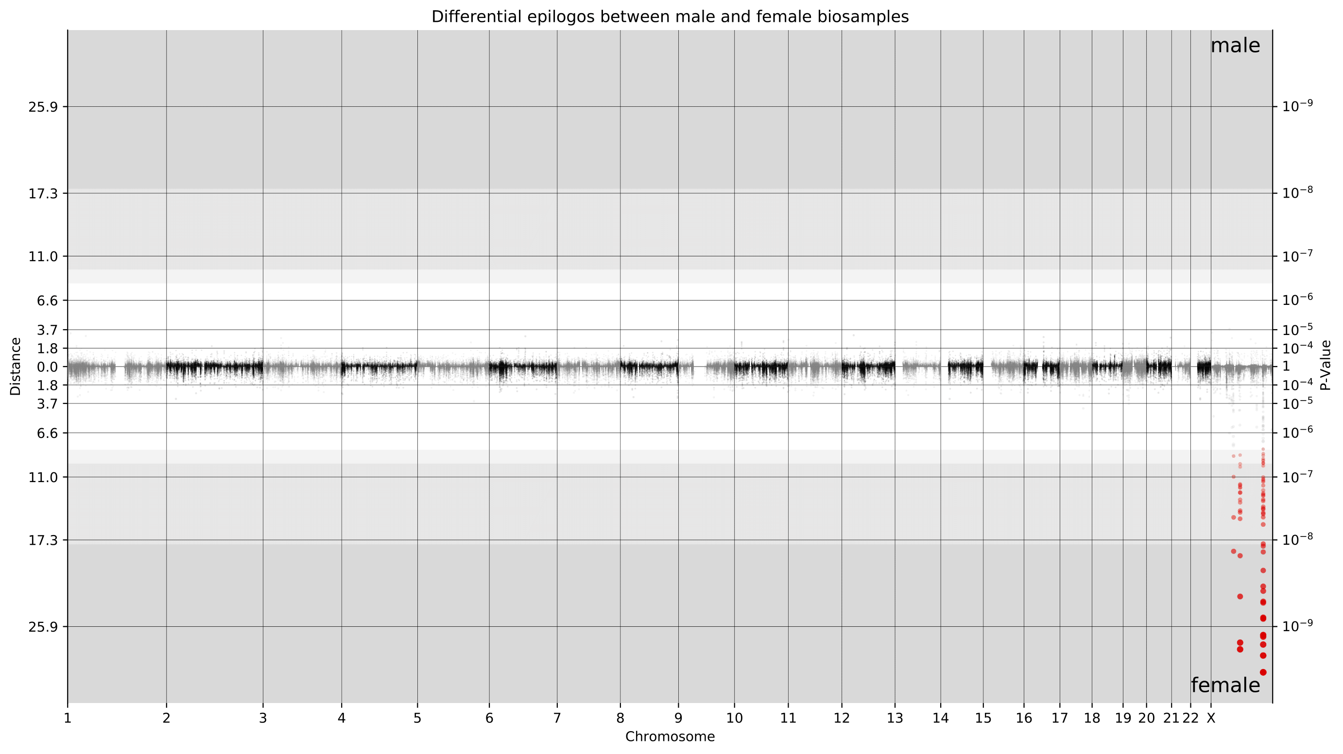
e.g. $ epilogos -g 30Unlike single group Epilogos, pairwise Epilogos has a visual component in the form of Manhattan-like plots.
Located in the manhattanPlots_* output directory, these plots offer users a way to visually locate differences between two groups of epigenomes.
Points are colored in case their scores have a z-score greater than 1. When using [-n, --null-distribution] points are colored in case they are found to be significantly different between groups, exceeding a threshold of 10% FDR.
The colors are as specified in the state info tsv provided by the user.
Additionally, points have varying opacity determined by the ratio of their distance to the most extreme distance.
The background color represents the z-score.
White indicates less than 10 and the shades of gray indicate greater than 10, 20, and 30 (with darker being a higher z-score).
When using [-n, --null-distribution], the background color represents level of signficicance.
White indicates insignificant and the shades of gray indicate significance at 10%, 5%, and 1% FDR (with darker being more significant).
The example plot below shows a genome-wide Manhattan plot generated by a pairwise Epilogos run of material from male donors versus female donors in the EpiMap dataset. This view makes it immediately clear that the vast majority of chromatin state differences between male and female biosamples is on the X chromosome.
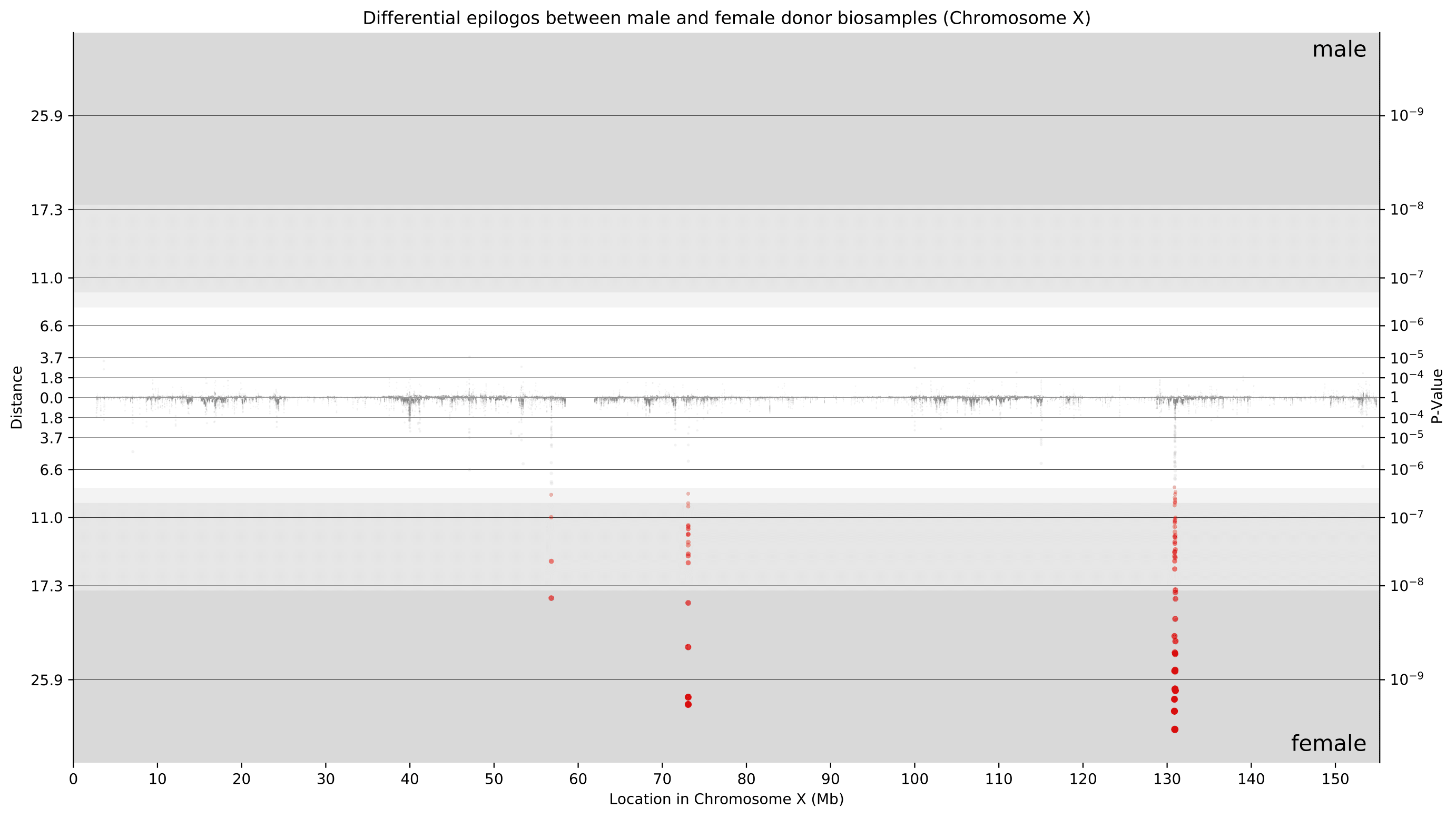
Considering that these differences are primarily present on chromosome X, we now can take a closer look at only chromosome X. With newfound granularity, we can begin to identify individual genes where differences are most pronounced. We can clearly see differences around 73 Mbp (XIST locus) and around 131 Mbp (FIRRE locus). Furthermore, the directionality of these points towards female donor biosamples indicates that these differences were driven by higher Epilogos scores in female donor biosamples. This is consistent with our knowledge of these loci playing crucial roles in the female-specific X-inactivation process.
Epilogos similarity search is a method to enhance the browsing experience of genome-wide epilogos datasets. Similarity search reduces an Epilogos dataset into a set non-overlapping regions and performs a nearest neighbor search to identify the highest similarity regions for each region.
To be presented with minimal documentation of arguments needed to run similarity search, simply run the command simsearch --help or python -m simsearch --help (More in-depth explanation is given below)
Due to its computationally intensive nature, calculating similarity search results requires a computational cluster managed by SLURM (as used in Epilogos score calculation). If you want to query previously calculated similarity search results, this can is done without a computational cluster, simply in the command line.
Minimal example on provided example data
If you cloned this git repository, example data has been provided under data/simsearch/male/. Otherwise it is available for download using the script in bin/download_example_data.sh. The script uses cURL to download neccessary files and places them in a file hierarchy generated within the current directory.
The file, named scores_male_s1_matrix_chr1.txt.gz, contains epilogos scores for a 18-state chromatin model, across 200bp genomic bins spanning human chromosome 1.
The data consist of epilogos scores calculated on chromosome 1 of the EpiMap dataset and contains only those epigenomes which are tagged Male under the Sex column.
To compute similarity search results for this sample data run the following command within the epilogos/ directory (replacing BUILD_OUTPUTDIR with the output directory of your choice).
$ simsearch -b -s data/simsearch/male/scores_male_s1_matrix_chr1.txt.gz -o BUILD_OUTPUTDIRUpon completion of the run, you should see the files simsearch_cube.npz, simsearch_indices.npy, reduced_genome.npy, simsearch.bed.gz, and simsearch.bed.gz.tbi in BUILD_OUTPUTDIR.
For further explanation of the contents of these outputs see Build Output Directory [-o, --output-directory]
To query the Similarity Search results for a given region run the following command (replacing CHR, START, & END with the region coordinates, BUILD_OUTPUTDIR with the build step output directory, and QUERY_OUTPUTDIR with the output directory of your choice).
$ simsearch -q CHR:START-END -m BUILD_OUTPUTDIR/simsearch.bed.gz -o QUERY_OUTPUTDIRUpon completion of the run, you should see the file similarity_search_region_CHR_START_END_recs.bed in QUERY_OUTPUTDIR.
For further explanation of the contents of these outputs see Query Output Directory [-o, --output-directory]
To customize your run of Similarity Search see the Command Line Options of the README
Running Similarity Search with your own data
Before you can run Similarity Search on your own data, you will first need an epilogos scores file. When epilogos is run, it outputs scores split by chromosome. Because Similarity Search can only read in one file, if you want to run similarity search across the whole genome, you will have to combine these files into one singular scores file. This file can have chromosomes sorted by genomic (i.e. chr9 before chr12) or lexicographic (i.e. chr12 before chr9) order. We recommend using the either of following commands:
Genomic:
$ prefix="PATH/TO/EPILOGOS_OUTPUT_DIR/scores_*"; suffix="txt.gz"; paths=""; for chr in GENOMIC_ORDER; do chr="chr${chr}"; path="${prefix}_${chr}.${suffix}"; paths="${paths} ${path}"; done; cat ${paths} > PATH/TO/EPILOGOS_OUTPUT_DIR/scores.txt.gzWhere is GENOMIC_ORDER is replaced with the names of the relevant chromosomes in order separated by spaces. (e.g. 1 2 3 4 5 6 7 8 9 10 11 12 13 14 15 16 17 18 19 20 21 22 X Y or `seq 1 22` X Y for humans)
Lexicographic (requires bedops):
$ zcat PATH/TO/EPILOGOS_OUTPUT_DIR/scores_*_chr*.txt.gz | sort-bed - > PATH/TO/EPILOGOS_OUTPUT_DIR/scores.txt; gzip PATH/TO/EPILOGOS_OUTPUT_DIR/scores.txtOnce you have your desired scores file you can generate Similarity Search results with the following command:
$ simsearch -b -s PATH/TO/EPILOGOS_SCORES_FILE -o PATH/TO/BUILD_OUTPUT_DIRUpon completion of the run, you should see the files simsearch_cube.npz, simsearch_indices.npy, reduced_genome.npy, simsearch.bed.gz, and simsearch.bed.gz.tbi in PATH/TO/BUILD_OUTPUT_DIR.
For further explanation of the contents of these outputs see Build Output Directory [-o, --output-directory]
To query these Similarity Search results for a given region run the following command (replacing CHR, START, & END with the region coordinates, PATH/TO/BUILD_OUTPUT_DIR with the build step output directory, and PATH/TO/BUILD_OUTPUT_DIR with the output directory of your choice).
$ simsearch -q CHR:START-END -m PATH/TO/BUILD_OUTPUT_DIR/simsearch.bed.gz -o PATH/TO/BUILD_OUTPUT_DIRUpon completion of the run, you should see the file similarity_search_region_CHR_START_END_recs.bed in PATH/TO/BUILD_OUTPUT_DIR.
For further explanation of the contents of these outputs see Query Output Directory [-o, --output-directory]
To further customize your run of epilogos see the Command Line Options of the README
Build Similarity Search Results [-b, --build]
The Similarity Search commandline interface has two modes: build and query. Build mode takes in a single epilogos scores file, finds regions of a specified size, and finds the best matches for each of these regions.
When -b is enabled, run Similarity Search in build mode
e.g. $ simsearch -bScores Path [-s, --scores-path]
In [-b, --build] mode, Similarity Search takes as input a single epilogos scores file. When epilogos is run, it outputs scores split by chromosome. Because Similarity Search can only read in one file, if you want to run similarity search across the whole genome, you will have to combine these files into one singular scores file. This file can have chromosomes sorted by genomic (i.e. chr9 before chr12) or lexicographic (i.e. chr12 before chr9) order. We recommend using the either of following commands:
Genomic:
$ prefix="PATH/TO/EPILOGOS_OUTPUT_DIR/scores_*"; suffix="txt.gz"; paths=""; for chr in GENOMIC_ORDER; do chr="chr${chr}"; path="${prefix}_${chr}.${suffix}"; paths="${paths} ${path}"; done; cat ${paths} > PATH/TO/EPILOGOS_OUTPUT_DIR/scores.txt.gzWhere is GENOMIC_ORDER is replaced with the names of the relevant chromosomes in order separated by spaces. (e.g. 1 2 3 4 5 6 7 8 9 10 11 12 13 14 15 16 17 18 19 20 21 22 X Y or `seq 1 22` X Y for humans)
Lexicographic (requires bedops):
$ zcat PATH/TO/EPILOGOS_OUTPUT_DIR/scores_*_chr*.txt.gz | sort-bed - > PATH/TO/EPILOGOS_OUTPUT_DIR/scores.txt; gzip PATH/TO/EPILOGOS_OUTPUT_DIR/scores.txtThe argument to this flag is the path to the file you would like to read data from.
e.g. $ simsearch -b -s data/simsearch/male/scores_male_s1_matrix_chr1.txt.gzOutput Directory [-o, --output-directory]
In [-b, --build] mode, Similarity Search will output 5 files: simsearch_cube.npz, simsearch_indices.npy, reduced_genome.npy, simsearch.bed.gz, and simsearch.bed.gz.tbi
simsearch_cube.npz is a zipped archive of 2 numpy arrays: scores and coords. scores contains the epilogos scores across each region present in the similarity search output (regions are chosen by the mean-max algorithm as outlined in the filter-regions package). Scores are condensed into 25 blocks regardless of chosen window size. Scores in each of these blocks consist of the epilogos scores of the bin with the highest sum of scores in each block. coords contains the coordinates for each region, and is sorted in the same order as scores.
simsearch_indices.npy is a numpy array file containing the similarity search results as indices of the reduced_genome.npy array (the index encodes the first of 25 superbins in the resulting region). Each line contains the results for the region of the same line in simsearch_cube.npz. If similarity search found less than [-n, --num-matches] matches for a region remaining indices in the row will consist of -1.
reduced_genome.npy is a numpy array file containing the reduced scores of the epilogos input file. Because similarity search always searches via regions consisting of 25 'superbin', scores are reduced by a factor dependent on the window size chosen.
simsearch.bed.gz is a gzipped bed file containing the coordinates of each region followed by the coordinates of its top [-n, --num-matches] matches.
simsearch.bed.gz.tbi is a tabix equivalent of simsearch.bed.gz.
The argument to this flag is the path to the directory to which you would like to output.
e.g. $ simsearch -b -s data/simsearch/male/scores_male_s1_matrix_chr1.txt.gz -o BUILD_OUTPUTDIR/Window Size [-w, --window-bp]
Similarity Search uses the mean-max algorithm outlined in the filter-regions package to divide the genome into non-overlapping regions of a user-specified size (prioritizing regions based on information content). Scores within these regions are condensed into 25 blocks regardless of chosen window size. Scores in each of these blocks consist of the epilogos scores of the bin with the highest sum of scores in each block.
Only a set number of window size options are available for Similarity Search. When run on a 200bp bin dataset, these are 5000, 10000, 25000, 50000, 75000, and 100000. When run on a 20bp bin dataset, these are 500, 1000, 2500, 5000, 7500, and 10000
The argument to this flag is the desired window size in bp (default = 25000 (200bp dataset) or 2500 (20bp dataset)).
e.g. $ simsearch -b -s data/simsearch/male/scores_male_s1_matrix_chr1.txt.gz -o OUTPUT_DIR -w 10000Number of Jobs [-j, --num-jobs]
Similarity Search submits SLURM jobs to distribute the burden of the euclidean distance calculation across different nodes.
The argument to this flag is the number of parallel slurm jobs to run for the euclidean distance calculation (default=10).
e.g. $ simsearch -b -s data/simsearch/male/scores_male_s1_matrix_chr1.txt.gz -o OUTPUT_DIR -j 4Number of Cores [-c, --num-cores]
Similarity Search will always try and parallelize the match calculation if it can. Computation done within each slurm job is parallelized using python's multiprocessing library
The argument to this flag is an integer number of cores you would like to utilize to perform this multiprocessing. Should you like to use all available cores, input 0 to the option (i.e. -c 0). Epilogos defaults to using 1 core.
e.g. $ simsearch -b -s data/simsearch/male/scores_male_s1_matrix_chr1.txt.gz -o OUTPUT_DIR -c 4Number of Matches [-n, --num-matches]
Similarity Search uses a running euclidean distance calculation to determine the best matches for each region. The argument to this flag is the number desired matches for each region (default=100).
e.g. $ simsearch -b -s data/simsearch/male/scores_male_s1_matrix_chr1.txt.gz -o OUTPUT_DIR -n 51Filter State [-f, --filter-state]
ChromHMM state models generally contain a 'quiescent state' which is not of functional interest. As such, to ease similarity search computation, we allow the user to set a filter state. When generating regions per the max-mean algorithm, similarity search filters out regions in which the max signial is from the filter state.
The argument to this flag is the integer representing the state you wish to filter upon. If set to 0, no filtering is done. By default similarity search filters upon the last state.
e.g. $ simsearch -b -s data/simsearch/male/scores_male_s1_matrix_chr1.txt.gz -o OUTPUT_DIR -f 12Filter Score [--filter-score]
To ease similarity search computation, we allow the user to set a filter score. When generating regions per the max-mean algorithm, similarity search filters out regions in which the max signial is less than the filter score.
The argument to this flag is a float representing scores below which you filter out. By default, no filtering is done on score (this is equivalent to setting the flag to -1)
e.g. $ simsearch -b -s data/simsearch/male/scores_male_s1_matrix_chr1.txt.gz -o OUTPUT_DIR --filter-score 1.3SLURM Partition [-p, --partition]
By default, Similarity Search uses the default partition designated by the system administrator to submit SLURM jobs. Use this flag if you would like to specify the partition for SLURM resource allocation.
The argument to this flag is the name of the partition on which you would like the SLURM jobs to run
e.g. $ simsearch -b -s data/simsearch/male/scores_male_s1_matrix_chr1.txt.gz -o OUTPUT_DIR -p queue0SLURM Job Tag [-t, --tag]
By default, Similarity Search jobs only contain the name of the python file they are running. Use this flag if you would like to add more information Similarity Search's job names.
The argument to this flag is a string you wish to add to Similarity Search's SLURM job names.
e.g. $ simsearch -b -s data/simsearch/male/scores_male_s1_matrix_chr1.txt.gz -o OUTPUT_DIR -t boix-hg38-18-s1Region Calculation Memory Allocation [--mm-mem]
This flag controls the amount of memory (in MB) assigned to the region calculation (max_mean) slurm job. Similarity search defaults to 10000
e.g. $ simsearch -b -s data/simsearch/male/scores_male_s1_matrix_chr1.txt.gz -o OUTPUT_DIR --mm-mem 8000Euclidean Distance Calculation Memory Allocation [--calc-mem]
This flag controls the amount of memory (in MB) assigned to each of the euclidean distance calculation (calc) slurm jobs. Similarity search defaults to 50000
e.g. $ simsearch -b -s data/simsearch/male/scores_male_s1_matrix_chr1.txt.gz -o OUTPUT_DIR --calc-mem 25000Writing Results Memory Allocation [--write-mem]
This flag controls the amount of memory (in MB) assigned to the slurm job (write) responsible for writing similarity search results to disk. Similarity search defaults to 5000
e.g. $ simsearch -b -s data/simsearch/male/scores_male_s1_matrix_chr1.txt.gz -o OUTPUT_DIR --write-mem 10000Query Similarity Search Results [-q, --query]
The Similarity Search commandline interface has two modes: build and query. Query mode takes in a region query(ies) and a previously calculated simsearch.bed.gz matches file and outputs the top [-n, --num-matches] matches for the query(ies).
The -q flag can handle both single & multi region queries. If querying a single region, the argument to the flag should be the region coordinates formatted as chr:start-end. If querying multiple regions, the argument to the flag should be the path to a tab-separated bed file.
e.g. $ simsearch -q chr4:93305800-93330800 -m /PATH/TO/simsearch.bed.gzor
e.g. $ simsearch -q /PATH/TO/query_regions.bed -m /PATH/TO/simsearch.bed.gzMatches File [-m, --matches-file]
In [-q, --query] mode, Similarity Search takes as argument a pre-built simsearch.bed.gz matches file (see build output for details). This file is queried to find the top [-n, --num-matches] matches for each of the query regions.
e.g. $ simsearch -q chr4:93305800-93330800 -m BUILD_OUTPUTDIR/simsearch.bed.gzOutput Directory [-o, --output-directory]
In [-q, --query] mode, Similarity Search will output 1 file for each query region: similarity_search_region_CHR_START_END_recs.bed (where CHR, START, & END are replaced with the query coordinates
similarity_search_region_CHR_START_END_recs.bed is a tab-separated bed file containing the coordinates for each of the top [-n, --num-matches] matches for the query region in sorted order.
The argument to this flag is the path to the directory to which you would like to output.
e.g. $ simsearch -q chr4:93305800-93330800 -m BUILD_OUTPUTDIR/simsearch.bed.gz -o QUERY_OUTPUTDIR/To modify a development version of epilogos, first set up a virtual environment via e.g. conda.
After activating the environment and installing dependencies, install epilogos in editable mode:
$ pip install -e .If you are using Mac OS X 11 (Big Sur) or later, it may be necessary to first install OpenBLAS, before installing Python dependencies that require it (such as scipy).
This can be done via Homebrew and setting environment variables to point to relevant library and header files:
$ brew install openblas
$ export SYSTEM_VERSION_COMPAT=1
$ export LAPACK=/usr/local/opt/openblas/lib
$ export LAPACK_SRC=/usr/local/opt/openblas/include
$ export BLAS=/usr/local/opt/openblas/lib
Then run pip install -e ., as before.