Welcome to NatUKE! Here we present usability explanations an explanation of our benchmark and some results. We also provide a preview of the data used in the experiments and the access to said data.
@INPROCEEDINGS{icsc2023natuke,
  author={Do Carmo, Paulo Viviurka and Marx, Edgard and Marcacini, Ricardo and Valli, Marilia and Silva e Silva, João Victor and Pilon, Alan},
  booktitle={2023 IEEE 17th International Conference on Semantic Computing (ICSC)},
  title={NatUKE: A Benchmark for Natural Product Knowledge Extraction from Academic Literature},
  year={2023},
  pages={199-203},
  doi={10.1109/ICSC56153.2023.00039}
}
NatUKE source code explanation for understanding, running and evaluating experiments.
(this source code breakdown is also the regular flow of execution from natuke)
Here we explain all the source code in the repository and the order in which to execute them:
clean_pdfs.ipynb: load pdfs considering database and prepare two dataframes to be used further;phrases_flow.py: load texts dataframe and separate the texts into 512 tokens phrases;topic_generation.ipynb: load phrases dataframe and create a topic cluster using BERTopic [4];topic_distribution.ipynb: load BERTopic model the phrases dataframe and distributes the topics filtering according to an upper limit of the proportion and outputs the dataframe;hin_generation.ipynb: load the filtered topics dataset and paper information to generate the usable knowledge graph;knn_dynamic_benchmark.py: runs the experiments using the generated knowledge graph, considering the parametrers set on the main portion of the code; (option for BiKE challenge (https://aksw.org/bike/))knn_dynamic_benchmark_splits.py: runs the experiments using the splits tailored for the BiKE (First International Biochemical Knowledge Extraction Challenge: http://aksw.org/bike/) challenge;dynamic_benchmark_evaluation.py: generates hits@k and mrr metrics for the experiments, allowing different parameters to be set for the algorithms used as well as the metrics;execution_time_processer.py: processes the dynamically.txtgenerated byknn_dynamic_benchmark.pyexperiments into a dataframe of execution times;metric_graphs.py: with the metric results and execution times allows the generation of personalized graphs;
natuke_utils.py: contains the source for the: methods; split algorithms; similar entity prediction; and metrics.exploration.ipynb: used to explore data, as for the quantities of each property.
All experiments were tested with a conda virtual environment of Python 3.8. With conda installed the virtual envs should be created with:
conda create --name [name] python=3.8
Install the requirements:
cd natuke
conda activate [name]
pip install -r requirements.txt
GraphEmbeddings
GraphEmbeddings submodule based on https://github.com/shenweichen/GraphEmbedding but the used algorithms works with tf 2.x
To install this version of GraphEmbeddings run:
cd GraphEmbeddings
python setup.py install
To run the benchmark execute knn_dynamic_benchmark.py after adding the repository with the data and adding the kg name in the code. Other parameters can also be changed within the code.
You can access a full KG and splits at: https://drive.google.com/drive/folders/1NXLQQsIXe0hz32KSOeSG1PCAzFLHoSGh?usp=sharing
Metapath2Vec
metapath2vec submodule based on: https://stellargraph.readthedocs.io/en/stable/demos/link-prediction/metapath2vec-link-prediction.html
For a better user experience we recommend setting up two virtual environments for running biologist:
requirements.txtfor all the codes, excepttopic_distribution.ipynb;topic_generation.ipynb; andhin_generation.ipynb;requirements_topic.txtfortopic_distribution.ipynb;topic_generation.ipynb; andhin_generation.ipynb(BERTopic requires a different numpy version for numba).
The files must follow a naming convention, for example knn_results_deep_walk_0.8_doi_bioActivity_0_2nd.csv:
knn_resultsis the name of the experiments batch used in natuke;deep_walkis the name of the algorithm;0.8represents the maximum train/test splits percentage in the evaluation stages;doi_bioActivityis the edge_type restored for evaluation;0is the random sampling for the splits;- and
2ndis the evaluation_stage.
All these parameters can be changed as needed in this portion of the dynamic_benchmark_evaluation.py
path = 'path-to-data-repository'
file_name = "knn_results"
splits = [0.8]
#edge_groups = ['doi_name', 'doi_bioActivity', 'doi_collectionSpecie', 'doi_collectionSite', 'doi_collectionType']
edge_group = 'doi_collectionType'
#algorithms = ['bert', 'deep_walk', 'node2vec', 'metapath2vec', 'regularization']
algorithms = ['deep_walk', 'node2vec', 'metapath2vec', 'regularization']
k_at = [1, 5, 10, 15, 20, 25, 30, 35, 40, 45, 50]
dynamic_stages = ['1st', '2nd', '3rd', '4th']
The problem of knowledge extraction from unstructured data sources is that authors may use different words or methods to describe the same thing. Using rule-based information extraction algorithms is therefore very challenging. In this work, we propose a benchmark and evaluate different ML embeddings to the task of unsupervised knowledge extraction. We design the evaluation as such that we measure the performance of each approach when inserting randomly selected portions of a crowd-sourced training data set.
In order to simulate a scenario whereas new training data is constantly added to the model, we removed all nodes that originated from the crowd-sourced data set out of the KG, leaving the papers connected only to their topics. The first train/test split consists of a 20/80% division, and for other stages, the train split is increased by 20% until it reaches an 80/20% division. We also enriched our KG with topics related to the papers using BERTopic [4]. In Figure 1 we present a visualization of the evaluation stages. In our benchmark, we evaluate the accuracy of each approach in predicting the resource from different chemical compound properties using hits@k. The metric hits@k calculates and average of how many predictions achieve top k rankings.
Figure 1 - evaluation stages

The data set used for evaluation as well as training was generated from hundreds of peer reviewed scientific articles where the information on more than 2,000 natural products were extracted. The data set was built manually by chemistry specialists that read the articles annotating four relevant properties associated with each natural product discussed in the paper: (I) metabolic class and (II) bioactivity, (III) species from where natural products were extracted, and (IV) collection site of this species.
The dataset can be found in different formats:
- Linked Data: http://nubbekg.aksw.org
- Spreadsheet: https://tinyurl.com/2p99u3jv
For the benchmark data was extracted from the linked data endpoint and then joined with the spreadsheet for missing values, with the following SPARQL query:
PREFIX rdf: <http://www.w3.org/1999/02/22-rdf-syntax-ns#>
PREFIX rdfs: <http://www.w3.org/2000/01/rdf-schema#>
PREFIX nubbe: <http://nubbe.db/>
PREFIX nubbeprop: <http://nubbe.db/property/>
PREFIX nubbeclass: <http://nubbe.db/class/>

SELECT DISTINCT
  ?doi ?bioActivity ?collectionSpecie ?collectionSite ?collectionType ?molType
  ?molecularMass ?monoisotropicMass ?cLogP ?tpsa?numberOfLipinskiViolations
  ?numberOfH_bondAcceptors ?numberOfH_bondDonors ?numberOfRotableBonds
  ?molecularVolume ?smile
WHERE {
  ?data     nubbeprop:doi                           ?doi                          .
  OPTIONAL {
    ?data   nubbeprop:biologicalActivity            ?bioActivity                  ;
            nubbeprop:collectionSpecie              ?collectionSpecie             ;
            nubbeprop:collectionSite                ?collectionSite               ;
            nubbeprop:collectionType                ?collectionType               ;
            rdf:type                                ?molType                      ;
            nubbeprop:molecularMass                 ?molecularMass                ;
            nubbeprop:monoisotropicMass             ?monoisotropicMass            ;
            nubbeprop:cLogP                         ?cLogP                        ;
            nubbeprop:tpsa                          ?tpsa                         ;
            nubbeprop:numberOfLipinskiViolations    ?numberOfLipinskiViolations   ;
            nubbeprop:numberOfH-bondAcceptors       ?numberOfH_bondAcceptors      ;
            nubbeprop:numberOfH-bondDonors          ?numberOfH_bondDonors         ;
            nubbeprop:numberOfRotableBonds          ?numberOfRotableBonds         ;
            nubbeprop:molecularVolume               ?molecularVolume              ;
            nubbeprop:smile                         ?smile                        .
  }
}
We compare four different unsupervised graph embedding methods for our knowledge extraction task: (1) DeepWalk is an unsupervised graph embedding method that uses random walks to sample a training data set for a skipgram architecture; (2) Node2Vec extends DeepWalk method to allow more control on the random walks; (3) Metapath2Vec is another extension from DeepWalk that transforms the random walks into meta-path based walks; and Embedding Propagation on Heterogeneous Networks (EPHEN) is an embedding propagation method that uses a regularization function to distribute an initial BERT embedding on a KG, meaning that it considers both text and structured data in an unsupervised scenario.
We use NubbeDB ontology (https://github.com/AKSW/dinobbio/tree/main/ontology) for property prediction. We extract five different properties: (1) name, (2) bioactivity, (3) specie, (4) collection site, and (5) isolation type. We use different values of k proportionally to the property-value prediction difficulty. For instance, it is significantly more challenging to predict the right natural product name than it is to predict the isolation type because there are considerable fewer exemplars in the traning data set for natural product than there is for isolation type. For that we evaluated with different k from 1 to 50, considering values multiples of 5.
The graphs show the results from experiments extracting five different natural product properties from biochemical academic papers. Each graph presents different property extraction and values of k to the hits@k metric: (1) name, k = 50; (2) bioactivity, k = 5; (3) specie, k = 50; (4) collection site, k = 20; and (5) isolation type, k = 1. The final k value for each extraction is defined either when a score higher than 0.50 is achieved at any evaluation stage or the upper limit of k = 50. The final k value for each extraction is defined either when a score higher than 0.50 is achieved at any evaluation stage or the upper limit of k = 50.
Graph 1 - compound name extraction

Graph 2 - bioactivity extraction

Graph 3 - collection specie extraction

Graph 4 - collection site extraction

Graph 5 - collection type extraction
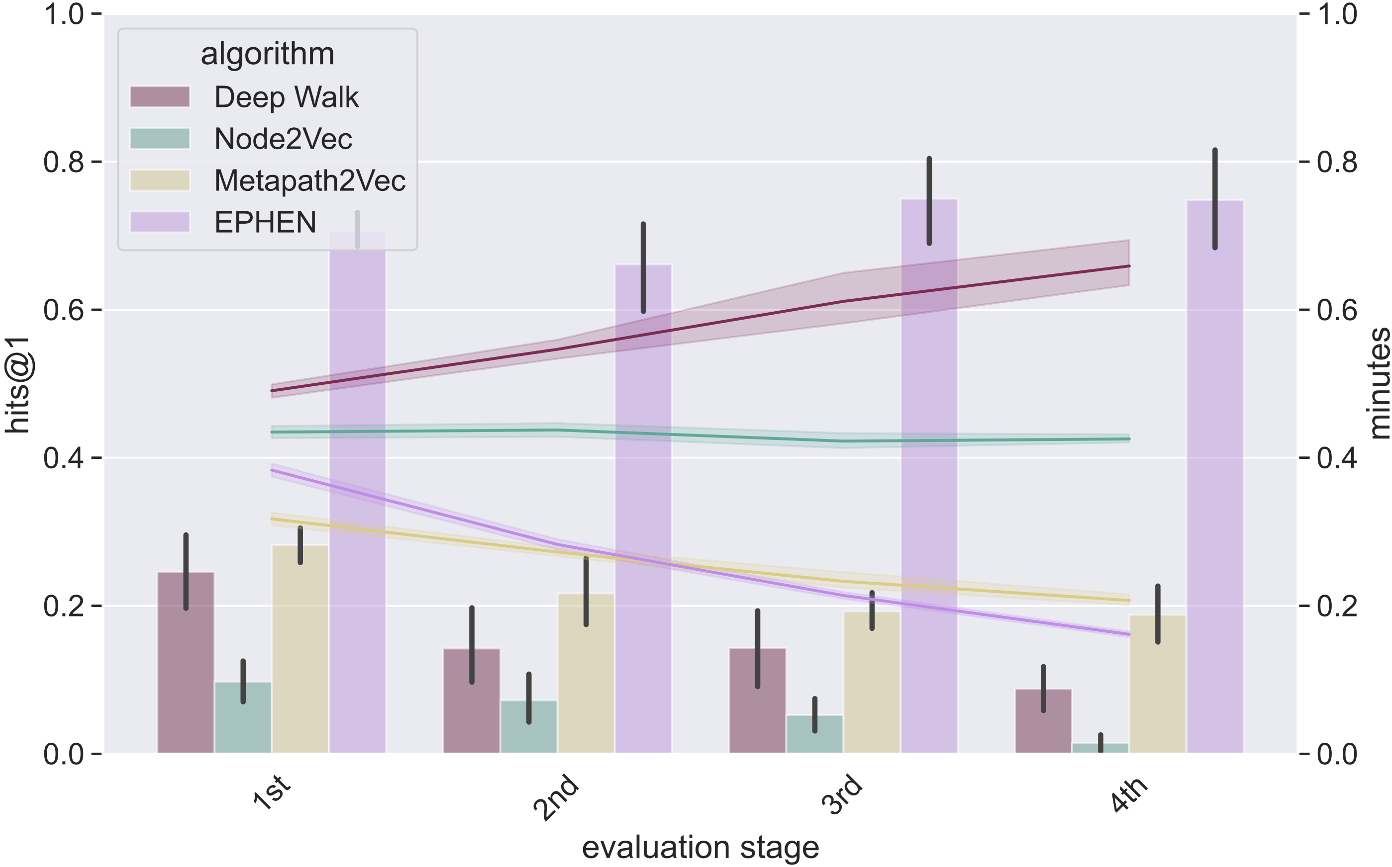
Table 1 shows the results from experiments extracting five different natural product properties from biochemical academic papers. They are presented on different values of k to the hits@k metric: (1) name, k = 50; (2) bioactivity, k = 5; (3) specie, k = 50; (4) collection site, k = 20; and (5) isolation type, k = 1. The final k value for each extraction is defined either when a score higher than 0.50 is achieved at any evaluation stage or the upper limit of k = 50.
Table 2 shows the results from experiments extracting five different natural product properties from biochemical academic papers. They are presented on different values of k to the hits@k metric: (1) name, k = 50; (2) bioactivity, k = 1; (3) specie, k = 20; (4) collection site, k = 5; and (5) isolation type, k = 1. The final k value for each extraction is defined either when a score higher than 0.20 is achieved at any evaluation stage or the upper limit of k = 50.
Table 1
Results table for extracting: chemical compound (C), bioactivity (B), specie (S), collection site (L), and isolation type (T). Performance metric with the average and standard deviation of the metric hits@k and k is respectively: 50, 5, 50, 20, and 1.
| Property | Evaluation Stage | DeepWalk | Node2vec | Metapath2Vec | EPHEN |
|---|---|---|---|---|---|
| C | 1st | 0.08 ± 0.01 | 0.08 ± 0.01 | 0.10 ± 0.01 | 0.09 ± 0.01 |
| 2nd | 0.01 ± 0.01 | 0.00 ± 0.01 | 0.08 ± 0.02 | 0.02 ± 0.01 | |
| 3rd | 0.01 ± 0.01 | 0.01 ± 0.01 | 0.09 ± 0.03 | 0.03 ± 0.02 | |
| 4th | 0.00 ± 0.00 | 0.00 ± 0.00 | 0.20 ± 0.05 | 0.04 ± 0.05 | |
| B | 1st | 0.41 ± 0.08 | 0.41 ± 0.07 | 0.27 ± 0.03 | 0.55 ± 0.06 |
| 2nd | 0.12 ± 0.02 | 0.07 ± 0.03 | 0.17 ± 0.06 | 0.57 ± 0.07 | |
| 3rd | 0.10 ± 0.03 | 0.03 ± 0.03 | 0.13 ± 0.04 | 0.60 ± 0.08 | |
| 4th | 0.07 ± 0.04 | 0.03 ± 0.03 | 0.12 ± 0.06 | 0.64 ± 0.07 | |
| S | 1st | 0.37 ± 0.04 | 0.36 ± 0.04 | 0.40 ± 0.03 | 0.36 ± 0.04 |
| 2nd | 0.24 ± 0.03 | 0.22 ± 0.03 | 0.41 ± 0.06 | 0.24 ± 0.03 | |
| 3rd | 0.27 ± 0.07 | 0.25 ± 0.06 | 0.42 ± 0.04 | 0.29 ± 0.07 | |
| 4th | 0.25 ± 0.10 | 0.24 ± 0.07 | 0.44 ± 0.12 | 0.30 ± 0.06 | |
| L | 1st | 0.56 ± 0.06 | 0.57 ± 0.05 | 0.40 ± 0.05 | 0.53 ± 0.03 |
| 2nd | 0.41 ± 0.05 | 0.36 ± 0.08 | 0.42 ± 0.04 | 0.52 ± 0.06 | |
| 3rd | 0.38 ± 0.06 | 0.28 ± 0.04 | 0.42 ± 0.08 | 0.55 ± 0.04 | |
| 4th | 0.29 ± 0.05 | 0.23 ± 0.10 | 0.40 ± 0.12 | 0.55 ± 0.06 | |
| T | 1st | 0.25 ± 0.09 | 0.10 ± 0.05 | 0.28 ± 0.04 | 0.71 ± 0.04 |
| 2nd | 0.14 ± 0.08 | 0.07 ± 0.06 | 0.22 ± 0.08 | 0.66 ± 0.10 | |
| 3rd | 0.14 ± 0.09 | 0.05 ± 0.04 | 0.19 ± 0.04 | 0.75 ± 0.10 | |
| 4th | 0.09 ± 0.05 | 0.01 ± 0.02 | 0.19 ± 0.06 | 0.75 ± 0.11 |
Table 2
Results table for extracting: chemical compound (C), bioactivity (B), specie (S), collection site (L), and isolation type (T). Performance metric with the average and standard deviation of the metric hits@k and k is respectively: 50, 1, 20, 5, and 1.
| Property | Evaluation Stage | DeepWalk | Node2vec | Metapath2Vec | EPHEN |
|---|---|---|---|---|---|
| C | 1st | 0.08 ± 0.01 | 0.08 ± 0.01 | 0.10 ± 0.01 | 0.09 ± 0.01 |
| 2nd | 0.01 ± 0.01 | 0.00 ± 0.01 | 0.08 ± 0.02 | 0.02 ± 0.01 | |
| 3rd | 0.01 ± 0.01 | 0.01 ± 0.01 | 0.09 ± 0.03 | 0.03 ± 0.02 | |
| 4th | 0.00 ± 0.00 | 0.00 ± 0.00 | 0.20 ± 0.05 | 0.04 ± 0.05 | |
| B | 1st | 0.10 ± 0.03 | 0.09 ± 0.04 | 0.06 ± 0.04 | 0.17 ± 0.05 |
| 2nd | 0.01 ± 0.01 | 0.02 ± 0.01 | 0.04 ± 0.03 | 0.19 ± 0.05 | |
| 3rd | 0.01 ± 0.01 | 0.01 ± 0.01 | 0.03 ± 0.02 | 0.24 ± 0.06 | |
| 4th | 0.01 ± 0.02 | 0.01 ± 0.01 | 0.10 ± 0.04 | 0.25 ± 0.06 | |
| S | 1st | 0.10 ± 0.03 | 0.10 ± 0.02 | 0.15 ± 0.02 | 0.10 ± 0.02 |
| 2nd | 0.12 ± 0.04 | 0.13 ± 0.03 | 0.11 ± 0.03 | 0.15 ± 0.03 | |
| 3rd | 0.12 ± 0.04 | 0.11 ± 0.05 | 0.15 ± 0.04 | 0.19 ± 0.05 | |
| 4th | 0.11 ± 0.06 | 0.11 ± 0.06 | 0.19 ± 0.07 | 0.22 ± 0.07 | |
| L | 1st | 0.15 ± 0.04 | 0.13 ± 0.04 | 0.12 ± 0.02 | 0.26 ± 0.04 |
| 2nd | 0.09 ± 0.03 | 0.08 ± 0.04 | 0.13 ± 0.04 | 0.29 ± 0.05 | |
| 3rd | 0.06 ± 0.03 | 0.06 ± 0.03 | 0.11 ± 0.04 | 0.30 ± 0.07 | |
| 4th | 0.06 ± 0.04 | 0.05 ± 0.03 | 0.13 ± 0.08 | 0.27 ± 0.07 | |
| T | 1st | 0.25 ± 0.09 | 0.10 ± 0.05 | 0.28 ± 0.04 | 0.71 ± 0.04 |
| 2nd | 0.14 ± 0.08 | 0.07 ± 0.06 | 0.22 ± 0.08 | 0.66 ± 0.10 | |
| 3rd | 0.14 ± 0.09 | 0.05 ± 0.04 | 0.19 ± 0.04 | 0.75 ± 0.10 | |
| 4th | 0.09 ± 0.05 | 0.01 ± 0.02 | 0.19 ± 0.06 | 0.75 ± 0.11 |
The code and experiments are available as open source under the terms of the Apache 2.0 License.
The dataset used for training and benchmark are available under the license Attribution-NonCommercial-NoDerivatives 4.0 International (CC BY-NC-ND 4.0). Which allows the use of the data only on its current form.
For and extended version of the paper and other information visit our wiki page: https://github.com/AKSW/natuke/wiki/NatUKE-Wiki.