gbif.range R package

gbif.range - An R package to generate species range maps based on ecoregions and a user-friendly GBIF wrapper

Status of the automatic CI R-CMD-check test

Although species ranges may be obtained using expert maps (e.g., IUCN and EUFORGEN) or modeling methods, expert data remains limited in the number of available species while applying models usually need more technical expertise, as well as many species observations.

When unavailable, such information may be extracted from the Global Biodiversity Information facility (GBIF), the largest public data repository inventorying georeferenced species observations worldwide (https://www.gbif.org/). However, retrieving GBIF records at large scale in R may be tedious, if users are unaware of the specific set of functions and parameters that need to be employed within the rgbif library, and because of the library's existing limitations on the number of downloaded records (<100'000) if no data request is made.

Here we present gbif.range, a R library that contains automated methods to generate species range maps from scratch using in-house ecoregions shapefiles and an easy-to-use GBIF download wrapper. Finally, this library also offers a set of additional very useful parameters and functions for large GBIF datasets (generate doi, extract GBIF taxonomy, records filtering...).

(source: globe image from the Noun Project adapted by LenaCassie-Studio)

Description

GBIF wrapper

One the one hand, get_gbif() is a wrapper which allows the whole observations of a given species scientific name (accepted and synonym names) to be automatically retrieved, and improves the data accessibility of the rgbif R package (CRAN). The user download hard limit of rgbif is a maximum of 100,000 of species observations in one go if the easy-to-use interactive functions occ_search() and occ_data() are used (i.e., if no official download request is made with occ_download(), see). This impends the fast accessibility to the GBIF database when large observational datasets for many species and regions of the world are needed, specifically in scientific fields related to macroecology, modelling or satellite imagery. get_gbif() therefore bypasses this limit by intuitively using geographic parameters from occ_data() in rgbif, the terra R package and by adopting a dynamic moving window process allowing the user's study area of interest to be automatically fragmented in several tiles that always include < 100,000 observations.

On the other hand, get_gbif() also implements easy-to-use preliminary filtering options implemented during the download so that users save post-processing time in data cleaning. 13 filters are available. One is set by default in get_gbif() (hasGeospatialIssue = FALSE) whereas the others can be chosen independently, including two that are based on the CoordinateCleaner R package (CRAN). It is important to note that, although a strong records filtering may be undertaken with get_gbif(), CoordinateCleaner includes a larger variety of options that should be checked and applied on get_gbif outputs.

Range function

get_range() estimates species ranges based on occurrence data (a get_gbif output or a set of coordinates) and ecoregions. Ecoregions cover relatively large areas of land or water, and contain characteristic, geographically distinct assemblages of natural communities sharing a large majority of species, dynamics, and environmental conditions. The biodiversity of flora, fauna and ecosystems that characterise an ecoregion tends to be distinct from that of other ecoregions.

The function first deletes outliers from the observation dataset and then creates a polygon (convex hull) with a user specified buffer around all the observations of one ecoregion. If there is only one observation in a ecoregion, a buffer around this point will be created. If all points in a ecoregion are on a line, the function will also create a buffer around these points, however, the buffer size increases with the number of points in the line. More details to come...

Additonal functions

gbif.range also includes a set of additional functions meant to be a nice supplement of the features and data that offer get_gbif and get_range:

• get_status(): Generates, based on a given species name, its IUCN red list status and a list of all scientific names (accepted, synonyms) found in the GBIF backbone taxonomy to download the data. Children and related doubtful names not used to download the data may also be extracted. The function allows therefore taxonomy correspondency to be made between different species and sub-species to potentially merge their records, but also permits efficient ways of linking external data of a species which is named differently across databases.
• obs_filter(): Whereas the 'grain' parameter in get_gbif() allows GBIF observations to be filtered according to a certain spatial precision, obs_filter() accepts as input a get_gbif() output (one or several species) and filter the observations according to a specific given grid resolution (one observation per pixel grid kept). This function allows the user to refine the density of GBIF observations according to a defined analysis/study's resolution.
• make_tiles(): May be used to generate a set of SpatialExtent and geometry arguments POLYGON() based on a given geographic extent. This function is meant to help users who want to use the rgbif R package and its parameter geometry that uses a POLYGON() argument.
• get_doi(): A small wrapper of derived_dataset() in rgbif that simplifies the obtention of a general DOI for a set of several gbif species datasets.
• make_ecoregion(): A function to create custom ecoregions based on environmental layers.

Installation

You can install the development version from GitHub with:

remotes::install_github("8Ginette8/gbif.range")
library(gbif.range)
library(terra)
library(rnaturalearth)

Example

Terrestrial species

Let's download worldwide the records of Panthera tigris only based on true observations:

# Download
obs.pt = get_gbif(sp_name="Panthera tigris",
                  basis=c("OBSERVATION","HUMAN_OBSERVATION","MACHINE_OBSERVATION"))

# Plot species records
countries = vect(ne_countries(type = "countries",returnclass = "sf"))
plot(countries,col="#bcbddc")
points(obs.pt[,c("decimalLongitude","decimalLatitude")],pch=20,col="#99340470",cex=1.5)

Note that an additional filtering needs here to be done as one observation is found in the 🔷US🔷. A lot of tigers are being captive in this country hence the recorded observation. Therefore using additional functions from CoordinateCleaner might solve this issue. We can also retrieve the tiger IUCN red list status, and its scientific names (accepted and synonyms) that were used in the download with the GBIF backbone taxonomy. If all = TRUE, additonal children and related doubtful names may also be extracted (not used in get_gbif()):

get_status("Panthera tigris",all=FALSE)

Let's now generate the distributional range map of Panthera tigris using the in-house shapefile of terresterial ecoregions (eco.earth):

range.tiger = get_range(sp_name="Panthera tigris",
                        occ_coord=obs.pt,
                        Bioreg=eco.earth,
                        Bioreg_name="ECO_NAME")

Let's plot the result now:

plot(countries,col="#bcbddc")
plot(range.tiger,col="#238b45",add=TRUE,axes=FALSE,legend=FALSE)

Interestingly no tiger range was found in the US. Our get_range default parameters allowed the one US record of Panthera tigris to be flagged and considered as an outlier. Note that five parameters need to be set in get_range and those should be carefully explored before any definite map process.

Available ecoregions

Although whatever shapefile may be set in get_range() as input, note that three ecoregion shapefiles are already included in the library: eco.earh (for terrestrial species; The Nature conservancy 2009 adapted from Olson & al. 2001), eco.marine (for marine species; The Nature Conservancy 2012 adapted from Spalding & al. 2007, 2012) and eco.fresh (for freshwater species; Abell & al. 2008). For marine species, eco.earth may also be used if the user wants to represent the terrestrial range of species that also partially settle on mainland. For fresh water species, same may be done if the user considers that terrestrial ecoregions should be more representtaive of the species ecology. Each ecoregion shapefile has one or more categories, which describe more or less precisely the ecoregion world distribution (from the more to the less detailed):

• eco.earth has three different levels: 'ECO_NAME', 'WWF_MHTNAM' and 'WWF_REALM2'.
• eco.fresh has only one: 'FEOW_ID'.
• eco.marine contains a mix of two types of marine ecoregions, with common ('PROVINC' and 'REALM') and distinct levels:

For PPOW (Pelagic provinces of the world): 'BIOME'.

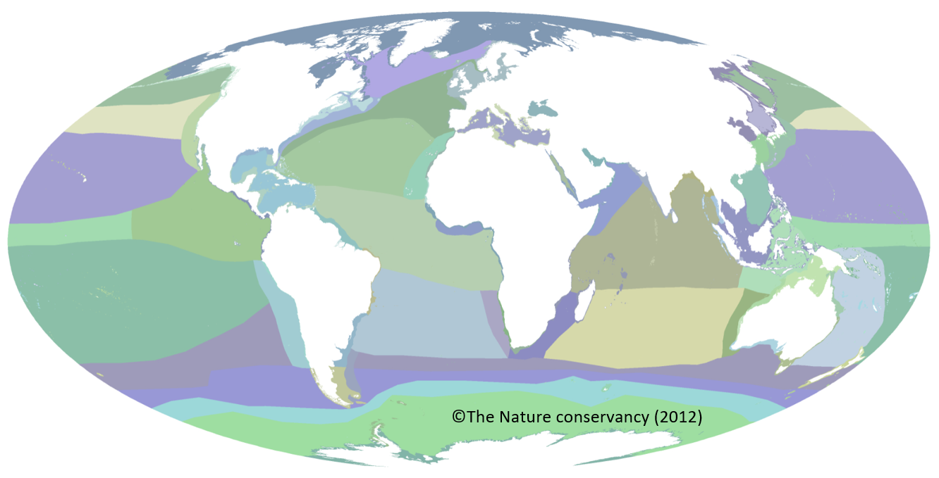
For MEOW (Marine ecoregions of the world): 'ECOREGION'.

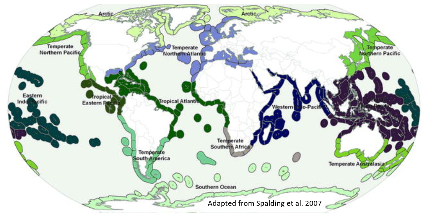
Note that a more detailed version of eco.marine (Marine Ecoregions and Pelagic Provinces of the World) may be found here. This version is available along eco.marine, and describes more detailed ecoregions along the coasts.

To access the polygon data in R:

data.frame(eco.earth)
data.frame(eco.fresh)
data.frame(eco.marine)

Which level should you pick depends on your questions and which level of the species' ecology you want to represent. Here, we chose eco.earth since Panthera tigris is of course a terrestrial species, and the very detailed 'ECO_NAME' as an ecoregion level because we wanted to obtain a more fine distribution.

Custom ecoregions

Additonally, if the in-house ecoregions are too coarse for a given geographic region (e.g., for local studies) or an ecoshapefile of finer environmental details is needed, make_ecoregion() can be used based on spatially-informed environment (e.g. climate) of desired resolution and extent defining the study area; example:

# Let's download the observations of Arctostaphylos alpinus in the European Alps:
shp.lonlat = vect(paste0(system.file(package = "gbif.range"),"/extdata/shp_lonlat.shp"))
obs.arcto = get_gbif("Arctostaphylos alpinus",geo=shp.lonlat)

# Create an ecoregion layer of 200 classes, based on 12 environmental spatial layers:
rst = rast(paste0(system.file(package = "gbif.range"),"/extdata/rst.tif"))
my.eco = make_ecoregion(rst,200)

# Create the range map based on our custom ecoregion
# (always set 'EcoRegion' as a name when using a make_ecoregion() output):
range.arcto = get_range(sp_name="Arctostaphylos alpinus",
                        occ_coord=obs.arcto,
                        Bioreg=my.eco,
                        Bioreg_name="EcoRegion",
                        res=20,
                        degrees_outlier = 5,
                        clustered_points_outlier = 2,
                        buffer_width_point = 4, 
                        buffer_increment_point_line = 0.5, 
                        buffer_width_polygon = 0.1)

Here we adapted the extra-parameters to the extent of the study area, e.g., (i) consider points as outliers (a maximum group of two points) if this bunch is away > 555km (1° ~ 111km) from the other cluster points and (ii) apply a buffer of ~10km around the drawn polygons. ⚠️It also important to note that the resolution parameter ('res') can be changed to adjust how fine the spatial output should be. This highest possible resolution will only depend on the precision of the Bioreg object (e.g., a range output can reach the same resolution of the rasters used to create a make_ecoregion object).

# Plot
plot(rst[[1]])
plot(shp.lonlat,add=TRUE)
plot(range.arcto,add=TRUE,col="darkgreen",axes=FALSE,legend=FALSE)
points(obs.arcto[,c("decimalLongitude","decimalLatitude")],pch=20,col="#99340470",cex=1)

Marine species

Let's reapply the same process as for Panthera tigris, but with the marine species Delphinus delphis (> 100'000 observations).

⚠️Notes that the download takes here longer unless the parameter occ_samp is used. Altough giving less precise observational distribution, occ_samp allows to extract a subsample of n GBIF observations per created tiles over the study area:

obs.dd = get_gbif("Delphinus delphis",occ_samp=1000) # Here the example is a sample of 1000 observations per geographic tile
get_status("Delphinus delphis",all=TRUE) # Here the list is longer because 'all=TRUE' includes every names (even doubtful)

Let's now generate three range maps of Delphinus delphis using eco.marine as ecoregion shapefile:

range.dd1 = get_range("Delphinus delphis",obs.dd,eco.marine,"PROVINC") # Coast and deep sea
range.dd2 = get_range("Delphinus delphis",obs.dd,eco.marine,"ECOREGION") # Coast only
range.dd3 = get_range("Delphinus delphis",obs.dd,eco.marine,"BIOME") # Deep sea only

The three results are pretty similar because most of the observations are near the coast. But let's plot the third result:

plot(countries,col="#bcbddc")
plot(range.dd3,col="#238b45",add=TRUE,axes=FALSE,legend=FALSE)
points(obs.dd[,c("decimalLongitude","decimalLatitude")],pch=20,col="#99340470",cex=1)

Althought our result map follows the sampling pattern found in GBIF, the dolphin range map might have been improved if more GBIF observations woud have been extracted. Therefore, occ_samp must be in this case increased or removed.

⚠️Finally, also note that in case of too many records, get_range can be used with a subsample of species observations to ensure a faster polygon process and/or to overcome potential RAM crashes.

Citation

Yohann Chauvier; Oskar Hagen; Camille Albouy; Patrice Descombes; Fabian Fopp; Michael P. Nobis; Philipp Brun; Lisha Lyu; Loïc Pellissier; Katalin Csilléry (2022). gbif.range - An R package to generate species range maps based on ecoregions and a user-friendly GBIF wrapper. EnviDat. doi: 10.16904/envidat.352

References

Oskar Hagen, Lisa Vaterlaus, Camille Albouy, Andrew Brown, Flurin Leugger, Renske E. Onstein, Charles Novaes de Santana, Christopher R. Scotese, Loïc Pellissier. (2019) Mountain building, climate cooling and the richness of cold-adapted plants in the Northern Hemisphere. Journal of Biogeography. doi: 10.1111/jbi.13653

Chauvier, Y., Thuiller, W., Brun, P., Lavergne, S., Descombes, P., Karger, D. N., ... & Zimmermann, N. E. (2021). Influence of climate, soil, and land cover on plant species distribution in the European Alps. Ecological monographs, 91(2), e01433. doi: 10.1002/ecm.1433

Lyu, L., Leugger, F., Hagen, O., Fopp, F., Boschman, L. M., Strijk, J. S., ... & Pellissier, L. (2022). An integrated high‐resolution mapping shows congruent biodiversity patterns of Fagales and Pinales. New Phytologist, 235(2), doi: 10.1111/nph.18158

Chamberlain, S., Oldoni, D., & Waller, J. (2022). rgbif: interface to the global biodiversity information facility API. doi: 10.5281/zenodo.6023735

Zizka, A., Silvestro, D., Andermann, T., Azevedo, J., Duarte Ritter, C., Edler, D., ... & Antonelli, A. (2019). CoordinateCleaner: Standardized cleaning of occurrence records from biological collection databases. Methods in Ecology and Evolution, 10(5), 744-751. doi: 10.1111/2041-210X.13152

Hijmans, Robert J. "terra: Spatial Data Analysis. R Package Version 1.6-7." (2022). Link to package: terra - CRAN

Olson, D. M., Dinerstein, E., Wikramanayake, E. D., Burgess, N. D., Powell, G. V. N., Underwood, E. C., D'Amico, J. A., Itoua, I., Strand, H. E., Morrison, J. C., Loucks, C. J., Allnutt, T. F., Ricketts, T. H., Kura, Y., Lamoreux, J. F., Wettengel, W. W., Hedao, P., Kassem, K. R. 2001. Terrestrial ecoregions of the world: a new map of life on Earth. Bioscience 51(11):933-938. doi: 10.1641/0006-3568(2001)051

The Nature Conservancy (2009). Global Ecoregions, Major Habitat Types, Biogeographical Realms and The Nature Conservancy Terrestrial Assessment Units. GIS layers developed by The Nature Conservancy with multiple partners, combined from Olson et al. (2001), Bailey 1995 and Wiken 1986. Cambridge (UK): The Nature Conservancy. Data URL: https://geospatial.tnc.org/datasets/b1636d640ede4d6ca8f5e369f2dc368b/about

Mark D. Spalding, Helen E. Fox, Gerald R. Allen, Nick Davidson, Zach A. Ferdaña, Max Finlayson, Benjamin S. Halpern, Miguel A. Jorge, Al Lombana, Sara A. Lourie, Kirsten D. Martin, Edmund McManus, Jennifer Molnar, Cheri A. Recchia, James Robertson, Marine Ecoregions of the World: A Bioregionalization of Coastal and Shelf Areas, BioScience, Volume 57, Issue 7, July 2007, Pages 573–583. doi: 10.1641/B570707

Spalding, M. D., Agostini, V. N., Rice, J., & Grant, S. M. (2012). Pelagic provinces of the world: a biogeographic classification of the world’s surface pelagic waters. Ocean & Coastal Management, 60, 19-30. doi: 10.1016/j.ocecoaman.2011.12.016

The Nature Conservancy (2012). Marine Ecoregions and Pelagic Provinces of the World. GIS layers developed by The Nature Conservancy with multiple partners, combined from Spalding et al. (2007) and Spalding et al. (2012). Cambridge (UK): The Nature Conservancy. Data URL: http://data.unep-wcmc.org/datasets/38

Robin Abell, Michele L. Thieme, Carmen Revenga, Mark Bryer, Maurice Kottelat, Nina Bogutskaya, Brian Coad, Nick Mandrak, Salvador Contreras Balderas, William Bussing, Melanie L. J. Stiassny, Paul Skelton, Gerald R. Allen, Peter Unmack, Alexander Naseka, Rebecca Ng, Nikolai Sindorf, James Robertson, Eric Armijo, Jonathan V. Higgins, Thomas J. Heibel, Eric Wikramanayake, David Olson, Hugo L. López, Roberto E. Reis, John G. Lundberg, Mark H. Sabaj Pérez, Paulo Petry, Freshwater Ecoregions of the World: A New Map of Biogeographic Units for Freshwater Biodiversity Conservation, BioScience, Volume 58, Issue 5, May 2008, Pages 403–414. doi: 10.1641/B580507