The documentation is being moved to here.
![]()
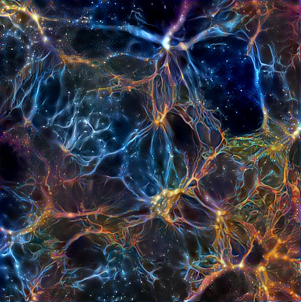
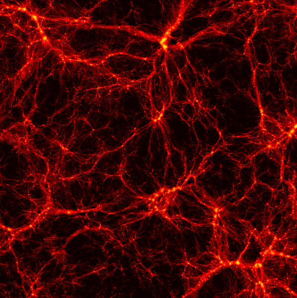
The image on the right have been generated by a neural network (DeepDream) from the image on the left
The Quijote simulations are a set of 43100 full N-body simulations. They are designed for two main tasks
- Quantify the information content on cosmological observables
- Provide enough statistics to train machine learning algorithms
But they can be used for a large variety of problems.
- Simulations run with the TreePM code Gadget-III
- More than 35 Million CPU hours
- Boxes of 1 Gpc/h. Combined total volume of 43100 (Gpc/h)^3 at a single redshift.
- 17100 simulations for a fiducial Planck cosmology
- Between 500 and 1000 simulations/cosmology for 17 different cosmologies
- 11000 simulations in different latin-hypercubes
- More than 8.5 trillions of particles at a single redshift
- Billions of halos and voids identified
- Full snapshots at redshifts 0, 0.5, 1, 2, 3 and 127 (initial conditions)
- More than 200000 halo catalogues
- More than 200000 void catalogues
- More than 1 million power spectra
- More than 1 million bispectra
- More than 1 million correlation functions
- More than 1 million marked power spectra
- More than 1 million probability distribution functions
- More than 1 Petabyte of data publicly available
The data is stored in the Gordon cluster of the San Diego Supercomputer Center. It can be access through globus.
- Log in into globus (create an account if you dont have one).
- Due to the volume of the data, the data is currently scattered across supercomputers in San Diego, New York and Princeton.
- To access the data in San Diego type: Quijote_simulations (or with this link)
- To access the data in New York type: Quijote_simulation2 (or with this link)
- To access the data in Princeton type: Princeton TIGRESS QUIJOTE Snapshots (or with this link)
Note that to download the data to your local machine (e.g. laptop) you will need to install the globus connect personal. For further details see here.
There are different folders:
- Snapshots. This folder contains the snapshots of the simulations
- Halos. This folder contains the halo catalogues
- Voids. This folder contains the void catalogues
- Linear_Pk. This folder contains the linear power spectra of each cosmological model
- Pk. This folder contains the power spectra
- Marked_Pk. This folder contains the marked power spectra
- Bk. This folder contains the bispectra
- CF. This folder contains the correlation functions
- PDF. This folder contains the pdfs
- density_field. This folder contains the 3D density fields
- density_field_2D. This folder contains the 2D density fields
Inside each of the above folders there is the data for the different cosmologies, e.g. h_p, fiducial, Om_m. A brief description of the different cosmologies is provided in the below table. Further details can be found in the Quijote paper.

The snapshots are stored in either Gadget-II format or HDF5. They can be read using the readgadget.py and readsnap.py scripts. If you have Pylians installed you already have them.
The snapshots only contain 4 blocks:
- Header: This block contains general information about the snapshot such as redshift, number of particles, box size, particle masses...etc.
- Positions: This block contains the positions of all particles. Stored as 32-floats
- Velocities: This block contains the velocities of all particles. Stored as 32-floats
- IDs: This block contains the IDs of all particles. Stored as 32-integers. (This block may be removed in the future to reduce the size of the snapshots)
An example on how to read a snapshot is this:
import readgadget

# input files
snapshot = '/home/fvillaescusa/Quijote/Snapshots/h_p/snapdir_002/snap_002'
ptype    = [1] #[1](CDM), [2](neutrinos) or [1,2](CDM+neutrinos)

# read header
header   = readgadget.header(snapshot)
BoxSize  = header.boxsize/1e3  #Mpc/h
Nall     = header.nall         #Total number of particles
Masses   = header.massarr*1e10 #Masses of the particles in Msun/h
Omega_m  = header.omega_m      #value of Omega_m
Omega_l  = header.omega_l      #value of Omega_l
h        = header.hubble       #value of h
redshift = header.redshift     #redshift of the snapshot
Hubble   = 100.0*np.sqrt(Omega_m*(1.0+redshift)**3+Omega_l)#Value of H(z) in km/s/(Mpc/h)

# read positions, velocities and IDs of the particles
pos = readgadget.read_block(snapshot, "POS ", ptype)/1e3 #positions in Mpc/h
vel = readgadget.read_block(snapshot, "VEL ", ptype)     #peculiar velocities in km/s
ids = readgadget.read_block(snapshot, "ID  ", ptype)-1   #IDs starting from 0
In the simulations with massive neutrinos it is possible to read the positions, velocities and IDs of the neutrino particles. Notice that the field should contain exactly 4 characters, that can be blank: "POS ", "VEL ", "ID ". The number in the name of the snapshot represents its redshift:
- 000 ------> z=3
- 001 ------> z=2
- 002 ------> z=1
- 003 ------> z=0.5
- 004 ------> z=0
The halo catalogues can be read through the readfof.py script. If you have Pylians installed you already have it. An example on how to read a halo catalogue is this:
import readfof

# input files
snapdir = '/home/fvillaescusa/Quijote/Halos/s8_p/145/' #folder hosting the catalogue
snapnum = 4                                            #redshift 0

# determine the redshift of the catalogue
z_dict = {4:0.0, 3:0.5, 2:1.0, 1:2.0, 0:3.0}
redshift = z_dict[snapnum]

# read the halo catalogue
FoF = readfof.FoF_catalog(snapdir, snapnum, long_ids=False,
                          swap=False, SFR=False, read_IDs=False)

# get the properties of the halos
pos_h = FoF.GroupPos/1e3            #Halo positions in Mpc/h
mass  = FoF.GroupMass*1e10          #Halo masses in Msun/h
vel_h = FoF.GroupVel*(1.0+redshift) #Halo peculiar velocities in km/s
Npart = FoF.GroupLen                #Number of CDM particles in the halo
The number in the name of the halo catalogue represents its redshift:
- 000 ------> z=3
- 001 ------> z=2
- 002 ------> z=1
- 003 ------> z=0.5
- 004 ------> z=0
The void catalogues are stored as hdf5 files. They contain the following blocks:
- pos: the positions of the void centers in Mpc/h
- radius: the sizes of the voids in in Mpc/h
- VSF: the void size function
- VSF_Rbins: the radii bins of the void size function
- parameters: the values of the void finder parameters used to generate the void catalogue
In python, the files can be read as
import h5py

f = h5py.File('/home/fvillaescusa/Quijote/Voids/fiducial/0/void_catalogue_m_z=0.hdf5', 'r')
pos        = f['pos'][:]        #void center positions in Mpc/h
radius     = f['radius'][:]     #void radii in Mpc/h
VSF        = f['VSF'][:]        #VSF (#voids/dR/Volume)
VSF_Rbins  = f['VSF_Rbins'][:]  #VSF radii in Mpc/h
parameters = f['parameters'][:] #parameters used to run the void finder

f.close()The different folders contain both the CAMB parameter files and the matter power spectrum at z=0. In some cases transfer functions and power spectra for neutrinos, CDM, baryons, and CDM+baryons are also present. The format of the power spectrum files is
- k | P(k)
where the units of k and P(k) are comoving h/Mpc and (Mpc/h)^3, respectively. For the fiducial, Om_p, Om_m, Ob_p, Ob_m, Ob2_p, Ob2_m, h_p, h_m, ns_p, ns_m, s8_p, s8_m the name of the matter power spectrum files at z=0 is 'CAMB_matterpow_0.dat'. For Mnu_p, Mnu_pp and Mnu_ppp the files are called instead 'XeV_Pm_rescaled_z0.0000.txt', where X = 0.1(Mnu_p), 0.2(Mnu_pp) and 0.4(Mnu_ppp). For the latin_hypercube simulations, the files are named 'Pk_mm_z=0.000.txt'
Notice that the matter power spectra at z=0 are not normalized (this is because the normalization is performed in the code that generates the initial conditions). The normalization factor is stored in the file Normfac.txt. One example on how to obtain the correct normalized matter power spectrum for a given cosmology is this:
import numpy as np

f_Pk   = '/home/fvillaescusa/Quijote/Linear_Pk/ns_p/CAMB_TABLES/CAMB_matterpow_0.dat'
f_norm = '/home/fvillaescusa/Quijote/Linear_Pk/ns_p/Normfac.txt'

k, Pk   = np.loadtxt(f_Pk, unpack=True)
Normfac = np.loadtxt(f_norm)

Pk_norm = Pk*np.sqrt(Normfac)The format of the power spectra are:
- k | P(k) for power spectra in real-space
- k | P0(k) | P2(k) | P4(k) for power spectra in redshift-space
where P0(k), P2(k) and P4(k) are the monopole, quadrupole and hexadecapole, respectively. The units of k are h/Mpc, while for the power spectra are (Mpc/h)^3.
In redshift-space there are three different files for each realization/redshift. These have been computed by placing the redshift-space distortions along the three different axes.
In python, the files can be read as
import numpy as np

k, Pk = np.loadtxt('/home/fvillaescusa/Quijote/Pk/matter/fiducial/3/Pk_m_z=0.txt', unpack=True)
k, Pk0, Pk2, Pk4 = np.loadtxt('/home/fvillaescusa/Quijote/Pk/matter/fiducial/3/Pk_m_RS1_z=0.txt', unpack=True)The files whose name starts with
- Mk_ contain marked power spectra M(k) evaluated at wavenumber k
- Xk_ contain the corss spectra between marked and standard density field X(k) evaluated at wavenumber k
The unit of k is h/Mpc, while the one of M(k) and X(k) is (Mpc/h)^3.
Files with measurements performed in the fiducial cosmology have name
- Mk_fiducial0-4999_....hdf5
- Xk_fiducial0-4999_....hdf5
where the first numbers (in the above case 0-4999) indicate the realizations saved in the file, and the dots specify the marked model considered.
The remaining files contain measurements performed in the other cosmologies and from 500 realization per cosmology. Their name is
- Mk_fTH_....hdf5
- Xk_fTH_....hdf5
Also in this case the dots specify the marked model considered.
In python, the files can be read as
import numpy as np

f = h5py.File(FILENAME, 'r')
k = f['k'][:]
# Fiducial cosmology
Mk = f['i'][:]
# Massive neutrino cosmologies
Mk = f['cosmo/i_suffix'][:]
# Other cosmologies
Mk = f['cosmo/i'][:]
where i is the number of the realization, cosmo is the wanted cosmology and suffix can be
- 'm' for the total matter field
- 'cb' for the cold dar matter plus baryons
In order to see the name of each cosmology type
print(list(f.keys()))
The format of the correlation functions are:
- R | xi(R) for correlation functions in real-space
- R | xi0(R) | xi2(R) | xi4(R) for correlation functions in redshift-space
where xi0(R), xi2(R) and xi4(R) are the monopole, quadrupole and hexadecapole, respectively. The units of R are Mpc/h, while the different xi are dimensionless.
In redshift-space there are three different files for each realization/redshift. These have been computed by placing the redshift-space distortions along the three different axes.
In python, the files can be read as
import numpy as np

R, xi = np.loadtxt('/home/fvillaescusa/Quijote/CF/matter/fiducial/0/CF_m_1024_z=0.txt', unpack=True)
R, xi0, xi2, xi4 = np.loadtxt('/home/fvillaescusa/Quijote/CF/matter/fiducial/0/CF_m_RS0_1024_z=0.txt', unpack=True)The format of the individual bispectra files are:
- k1/kf | k2/kf | k3/kf | P0(k1) | P0(k2) | P0(k3) | B0(k1,k2,k3) | Q(k1,k2,k3) | B_SN(k1,k2,k3) | counts
where k1, k2, k3 specify the length of the triangle sides, P0(k) is the power spectrum monopole, B0(k1,k2,k3) is the bispectrum monopole, Q(k1,k2,k3) is the reduced bipsectrum, B_SN is the bispectrum shot noise correction, and counts is the number of triangles in the bin. B0 is already shot noise corrected. The header specifies kf, the fundamental mode, and Nhalo, the number of halos.
The individual bispectra files can be read in python as follows,
import numpy as np

k1, k2, k3, p0k1, p0k2, p0k3, b123, q123, b_sn, cnts = np.loadtxt(FILENAME, skiprows=1, unpack=True, usecols=range(10))

# read header to get Nhalo
hdr = open(FILENAME).readline().rstrip()
Nhalo = int(hdr.split('Nhalo=')[-1])
Alternatively, sets of bispectra files for a specific redshift and cosmology can easily be accessed
import h5py

fbk = h5py.File(FILENAME, 'r')
k1 = fbk['k1'][...]
k2 = fbk['k2'][...]
k3 = fbk['k3'][...]
p0k1 = fbk['p0k1'][...]
p0k2 = fbk['p0k2'][...]
p0k3 = fbk['p0k3'][...]
b123 = fbk['b123'][...]
q123 = fbk['q123'][...]
b_sn = fbk['b_sn'][...]
cnts = fbk['counts'][...] # triange counts
Nhalos = fbk['Nhalos'][...] # number of halos
files = fbk['files'][...] # names of individual files. The format of the PDF files are:
- delta | pdf
where delta is the density contrast (rho/< rho > - 1).
In python, the files can be read as
import numpy as np

delta, pdf = np.loadtxt('/home/fvillaescusa/Quijote/PDF/matter/latin_hypercube/0/PDF_m_5.0_z=0.txt', unpack=True)- Francisco Villaescusa-Navarro (Flatiron/Princeton)
- ChangHoon Hahn (Berkeley)
- Elena Massara (Flatiron/Waterloo)
- Arka Banerjee (Stanford)
- Ana Maria Delgado (CUNY/Flatiron)
- Doogesh K. Ramanah (Sorbonne, Paris)
- Tom Charnock (Sorbonne, Paris)
- Elena Giusarma (Flatiron/MTech)
- Yin Li (Berkeley/IPMU)
- Erwan Allys (ENS, Paris)
- Antoine Brochard (ENS, Paris)
- Cora Uhlemann (Cambridge)
- Chi-Ting Chiang (BNL)
- Siyu He (Flatiron)
- Alice Pisani (Princeton)
- Andrej Obuljen (Waterloo)
- Yu Feng (Berkeley)
- Emanuele Castorina (Berkeley)
- Gabriella Contardo (Flatiron)
- Christina D. Kreisch (Princeton)
- Andrina Nicola (Princeton)
- Justin Alsing (Oskar Klein/Flatiron)
- Roman Scoccimarro (NYU)
- Licia Verde (Barcelona)
- Matteo Viel (SISSA)
- Shirley Ho (Flatiron/Princeton)
- Stephane Mallat (ENS/College de France)
- Ben Wandelt (IAP, Paris)
- David Spergel (Flatiron/Princeton)
For support, please send us an email at fvillaescusa@princeton.edu.